Return to Answer

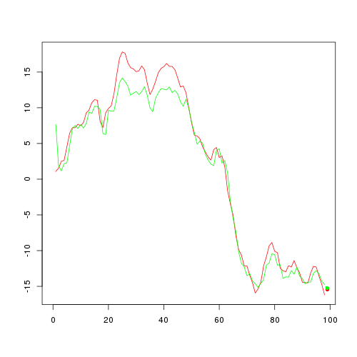
So what we did with the code is as follows. First, we have created a time-series example (from the ARIMA model). After that we have decoupled/sliced the time-series example into inputs of the form (sw previous points, next point) for all pairs except the last one (with the next point as the last point of the time-series example). The parameter sw is used to define the "sliding window". I won't debate here what is the proper size for the sliding-window but just note that due to Elman networks having memory the sliding-window of size one is more than a reasonable approach (also, take a look at this post).

So what we did with the code is as follows. First, we have created a time-series example (from the ARIMA model). After that we have decoupled/sliced the time-series example into inputs of the form (sw previous points, next point) for all pairs except the last one (with the next point as the last point of the time-series example). The parameter sw is used to define the "sliding window". I won't debate here what is the proper size for the sliding-window but just note that due to Elman networks having memory the sliding-window of size one is more than a reasonable approach (also, take a look at this post).

After the preparations are done we can simply build an Elman network with the elman function. There are two parameters you should be careful about; the size and the learnFuncParams. The size parameter gives you a way to define the size of the network (hidden layer) and the way you choose this parameter is more an art than a science. Rule of the thumb for learnFuncParams is to keep it small if it is feasible (your processing power allows you to keep it small/you have enough time to wait :D).

This was an example on how to use RNNs (Elman networks) with R to make predictons/forecasting. Some might argue that RNNs are not the best for the problem and that there are better nnet models for forecasting. Since I'm not an expert in the filed I will avoid discussing these issues.

After the preparations are done we can simply build an Elman network with the elman function. There are two parameters you should be careful about; the size and the learnFuncParams. The size parameter gives you a way to define the size of the network (hidden layer) and the way you choose this parameter is more an art than a science. A rule of thumb for learnFuncParams is to keep it small if it is feasible (your processing power allows you to keep it small/you have enough time to wait :D).

This was an example on how to use RNNs (Elman networks) with R to make predictions/forecasting. Some might argue that RNNs are not the best for the problem and that there are better nnet models for forecasting. Since I'm not an expert in the filed I will avoid discussing these issues.

library(RSNNS)

#
# simulate an arima time series example of the length n
#
set.seed(10001)
n <- 100
ts.sim <- arima.sim(list(order = c(1,1,0), ar = 0.7), n = n-1)

#
# create an input data set for ts.sim
# sw = sliding-window size
#
# the last point of the time series will not be used
#   in the training phase, only in the prediction/validation phase
# 
sw <- 1
X <- lapply(sw:(n-2),
       function(ind){
           ts.sim[(ind-sw+1):ind]
       })
X <- do.call(rbind, X)
Y <- sapply(sw:(n-2),
       function(ind){
           ts.sim[ind+1]
       })

# used to validate prediction properties
# on the last point of the series
newX <- ts.sim[(n-sw):(n-1)]
newY <- ts.sim[n]

# build an elman network besd on the input
model <- elman(X, Y,
               size = c(10, 10),
               learnFuncParams = c(0.001),
               maxit = 500,
               linOut = TRUE)

#
# plot the results
#
limits <- range(c(Y, model$fitted.values))

plot(Y, type = "l", col="red",
     ylim=limits, xlim=c(0, length(Y)),
     ylab="", xlab="")
lines(model$fitted.values, col = "green", type="l")

points(length(Y)+1, newY, col="red", pch=16)
points(length(Y)+1, predict(model, newdata=newX),
       pch="X", col="green")

This code should results in the following figure

library(RSNNS)

#
# simulate an arima time series example of the length n
#
set.seed(10001)
n <- 100
ts.sim <- arima.sim(list(order = c(1,1,0), ar = 0.7), n = n-1)

#
# create an input data set for ts.sim
# sw = sliding-window size
#
# the last point of the time series will not be used
#   in the training phase, only in the prediction/validation phase
# 
sw <- 1
X <- lapply(sw:(n-2),
       function(ind){
           ts.sim[(ind-sw+1):ind]
       })
X <- do.call(rbind, X)
Y <- sapply(sw:(n-2),
       function(ind){
           ts.sim[ind+1]
       })

# used to validate prediction properties
# on the last point of the series
newX <- ts.sim[(n-sw):(n-1)]
newY <- ts.sim[n]

# build an elman network based on the input
model <- elman(X, Y,
               size = c(10, 10),
               learnFuncParams = c(0.001),
               maxit = 500,
               linOut = TRUE)

#
# plot the results
#
limits <- range(c(Y, model$fitted.values))

plot(Y, type = "l", col="red",
     ylim=limits, xlim=c(0, length(Y)),
     ylab="", xlab="")
lines(model$fitted.values, col = "green", type="l")

points(length(Y)+1, newY, col="red", pch=16)
points(length(Y)+1, predict(model, newdata=newX),
       pch="X", col="green")

This code should result in the following figure