added 37 characters in body
Source Link
kjetil b halvorsen
  • 82.8k
  • 32
  • 201
  • 663
phone <-  read.table(file="phone.txt", header=TRUE)
library(reldist)
men  <-  phone[, 1]
women <-  phone[, 3]
reldist(men, women)
title("length of mens last phonecall with women as reference")
    phone <-  read.table(file="phone.txt", header=TRUE)
    library(reldist)
    men  <-  phone[, 1]
    women <-  phone[, 3]
    reldist(men, women)
    title("length of men's last phonecall with women as reference")
reldist(men, women, ci=TRUE)
title("length of mens last phonecall with women as reference\nwith pointwise confidence interval (95%)")
    reldist(men, women, ci=TRUE)
    title("length of men's last phonecall with women as 
           reference\nwith pointwise confidence interval (95%)")

Some more details about the relative density. Let $Q_0$ be the quantile function corresponding to $F_0$. Let $r$ be a quantile of $R$ with $y_r$ the corresponding value on the original measurement scale. Then the relative density can be written as $$ g(r) = \frac{f(Q_0(r))}{f_0(Q_0(r))} $$ or on the original measurement scale as $g(r)=\frac{f(y_r)}{f_0(y_r)}$. This shows that the relative density can be interpreted as a ratio of densities. But, in the first form, with argument $r$, it is also a density in own right, integrating to one over the interval $(0,1)$. That

That makes it a good starting point for inference.

phone <-  read.table(file="phone.txt", header=TRUE)
library(reldist)
men  <-  phone[, 1]
women <-  phone[, 3]
reldist(men, women)
title("length of mens last phonecall with women as reference")
reldist(men, women, ci=TRUE)
title("length of mens last phonecall with women as reference\nwith pointwise confidence interval (95%)")

Some more details about the relative density. Let $Q_0$ be the quantile function corresponding to $F_0$. Let $r$ be a quantile of $R$ with $y_r$ the corresponding value on the original measurement scale. Then the relative density can be written as $$ g(r) = \frac{f(Q_0(r))}{f_0(Q_0(r))} $$ or on the original measurement scale as $g(r)=\frac{f(y_r)}{f_0(y_r)}$. This shows that the relative density can be interpreted as a ratio of densities. But, in the first form, with argument $r$, it is also a density in own right, integrating to one over the interval $(0,1)$. That makes it a good starting point for inference.

    phone <-  read.table(file="phone.txt", header=TRUE)
    library(reldist)
    men  <-  phone[, 1]
    women <-  phone[, 3]
    reldist(men, women)
    title("length of men's last phonecall with women as reference")
    reldist(men, women, ci=TRUE)
    title("length of men's last phonecall with women as 
           reference\nwith pointwise confidence interval (95%)")

Some more details about the relative density. Let $Q_0$ be the quantile function corresponding to $F_0$. Let $r$ be a quantile of $R$ with $y_r$ the corresponding value on the original measurement scale. Then the relative density can be written as $$ g(r) = \frac{f(Q_0(r))}{f_0(Q_0(r))} $$ or on the original measurement scale as $g(r)=\frac{f(y_r)}{f_0(y_r)}$. This shows that the relative density can be interpreted as a ratio of densities. But, in the first form, with argument $r$, it is also a density in own right, integrating to one over the interval $(0,1)$.

That makes it a good starting point for inference.

added 8 characters in body
Source Link
Nick Cox
  • 59.5k
  • 8
  • 136
  • 212

There is a concept specifically for comparing distributions, which ought to be better known: the relative distribution.

LetsLet's say we have random variables $Y_0, Y$ with cumulative distribution functions $F_0, F$ and we want to compare them, using $F_0$ as a reference.

Define $$ R = F_0(Y) $$ The distribution of the random variable $R$ is the relative distribution of $Y$, with $Y_0$ as reference. Note that we have that $F_0(Y_0)$ has always the uniform distribution (with continuous random variables, if the random variables are discrete this will be approximate).

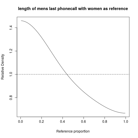
Let us look at an example. The website http://www.math.hope.edu/swanson/data/cellphone.txt gives data on the length of male and female studentsstudents' last phone call. Let us express the distribution of phone call length for male students, with women students as reference.
Relative distribution of phone call length, men compared to womenRelative distribution of phone call length, men compared with women

We can see immediately that men (in this college class ...) tend to have shorter phone calls than women ... and this is expressed directly, in a very direct way. On the $x$ axis is shown the proportions in the women's distribution, and we can read that, for example, for the time $T$ (whatever it is, its value is not shown) such that 20% of women's calls were shorter (or equal) to that, the relative density for men in that interval varies between about 1.3-1 and 1.4 about. If we approximate (mentally from the graph) the mean relative density in that interval as 1.35, we see that the proportion of men in that interval is about 35% higher than the proportion of women. That corresponds to 27% of the men in that interval.

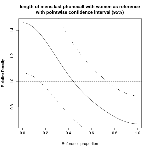
We can also make the same plot with pointwise confidence intervals around the relative density curve:
plot of relative distribution with pointwise confidence interval

The wide confidence bands in this case reflects the small sample size.

There is a book about this method: Handcock

The R code for the plot is here:

phone <-  read.table(file="phone.txt", header=TRUE)
library(reldist)
men  <-  phone[, 1]
women <-  phone[, 3]
reldist(men, women)
title("length of mens last phonecall with women as reference")

For the last plot change to:

reldist(men, women, ci=TRUE)
title("length of mens last phonecall with women as reference\nwith pointwise confidence interval (95%)")

Note that the plots are produced with use of kernel density estimation, with degree of smoothness chosen via gcv (generalized cross validation).

Some more details about the relative density. Let $Q_0$ be the quantile function corresponding to $F_0$. Let $r$ be a quantile of $R$ with $y_r$ the corresponding value on the original measurement scale. Then the relative density can be written as $$ g(r) = \frac{f(Q_0(r))}{f_0(Q_0(r))} $$ or on the original measurement scale as $g(r)=\frac{f(y_r)}{f_0(y_r)}$. This shows that the relative density can be interpreted as a ratio of densities. But, in the first form, with argument $r$, it is also a density in own right, integrating to one over the interval $(0,1)$. That makes it a good starting point for inference.

There is a concept specifically for comparing distributions, which ought to be better known: the relative distribution.

Lets say we have random variables $Y_0, Y$ with cumulative distribution functions $F_0, F$ and we want to compare them, using $F_0$ as a reference.

Define $$ R = F_0(Y) $$ The distribution of the random variable $R$ is the relative distribution of $Y$, with $Y_0$ as reference. Note that we have that $F_0(Y_0)$ has always the uniform distribution (with continuous random variables, if the random variables are discrete this will be approximate).

Let us look at an example. The website http://www.math.hope.edu/swanson/data/cellphone.txt gives data on the length of male and female students last phone call. Let us express the distribution of phone call length for male students, with women students as reference.

Relative distribution of phone call length, men compared to women

We can see immediately that men (in this college class ...) tend to have shorter phone calls than women ... and this is expressed directly, in a very direct way. On the $x$ axis is shown the proportions in the women's distribution, and we can read that, for example, for the time $T$ (whatever it is, its value is not shown) such that 20% of women's calls were shorter (or equal) to that, the relative density for men in that interval varies between 1.3-1.4 about. If we approximate (mentally from the graph) the mean relative density in that interval as 1.35, we see that the proportion of men in that interval is about 35% higher than the proportion of women. That corresponds to 27% of the men in that interval.

We can also make the same plot with pointwise confidence intervals around the relative density curve:

plot of relative distribution with pointwise confidence interval

The wide confidence bands in this case reflects the small sample size.

There is a book about this method: Handcock

The R code for the plot is here:

phone <-  read.table(file="phone.txt", header=TRUE)
library(reldist)
men  <-  phone[, 1]
women <-  phone[, 3]
reldist(men, women)
title("length of mens last phonecall with women as reference")

For the last plot change to:

reldist(men, women, ci=TRUE)
title("length of mens last phonecall with women as reference\nwith pointwise confidence interval (95%)")

Note that the plots are produced with use of kernel density estimation, with degree of smoothness chosen via gcv (generalized cross validation).

Some more details about the relative density. Let $Q_0$ be the quantile function corresponding to $F_0$. Let $r$ be a quantile of $R$ with $y_r$ the corresponding value on the original measurement scale. Then the relative density can be written as $$ g(r) = \frac{f(Q_0(r))}{f_0(Q_0(r))} $$ or on the original measurement scale as $g(r)=\frac{f(y_r)}{f_0(y_r)}$. This shows that the relative density can be interpreted as a ratio of densities. But, in the first form, with argument $r$, it is also a density in own right, integrating to one over the interval $(0,1)$. That makes it a good starting point for inference.

There is a concept specifically for comparing distributions, which ought to be better known: the relative distribution.

Let's say we have random variables $Y_0, Y$ with cumulative distribution functions $F_0, F$ and we want to compare them, using $F_0$ as a reference.

Define $$ R = F_0(Y) $$ The distribution of the random variable $R$ is the relative distribution of $Y$, with $Y_0$ as reference. Note that we have that $F_0(Y_0)$ has always the uniform distribution (with continuous random variables, if the random variables are discrete this will be approximate).

Let us look at an example. The website http://www.math.hope.edu/swanson/data/cellphone.txt gives data on the length of male and female students' last phone call. Let us express the distribution of phone call length for male students, with women students as reference.

Relative distribution of phone call length, men compared with women

We can see immediately that men (in this college class ...) tend to have shorter phone calls than women ... and this is expressed directly, in a very direct way. On the $x$ axis is shown the proportions in the women's distribution, and we can read that, for example, for the time $T$ (whatever it is, its value is not shown) such that 20% of women's calls were shorter (or equal) to that, the relative density for men in that interval varies between about 1.3 and 1.4. If we approximate (mentally from the graph) the mean relative density in that interval as 1.35, we see that the proportion of men in that interval is about 35% higher than the proportion of women. That corresponds to 27% of the men in that interval.

We can also make the same plot with pointwise confidence intervals around the relative density curve:

plot of relative distribution with pointwise confidence interval

The wide confidence bands in this case reflects the small sample size.

There is a book about this method: Handcock

The R code for the plot is here:

phone <-  read.table(file="phone.txt", header=TRUE)
library(reldist)
men  <-  phone[, 1]
women <-  phone[, 3]
reldist(men, women)
title("length of mens last phonecall with women as reference")

For the last plot change to:

reldist(men, women, ci=TRUE)
title("length of mens last phonecall with women as reference\nwith pointwise confidence interval (95%)")

Note that the plots are produced with use of kernel density estimation, with degree of smoothness chosen via gcv (generalized cross validation).

Some more details about the relative density. Let $Q_0$ be the quantile function corresponding to $F_0$. Let $r$ be a quantile of $R$ with $y_r$ the corresponding value on the original measurement scale. Then the relative density can be written as $$ g(r) = \frac{f(Q_0(r))}{f_0(Q_0(r))} $$ or on the original measurement scale as $g(r)=\frac{f(y_r)}{f_0(y_r)}$. This shows that the relative density can be interpreted as a ratio of densities. But, in the first form, with argument $r$, it is also a density in own right, integrating to one over the interval $(0,1)$. That makes it a good starting point for inference.

added 66 characters in body
Source Link
kjetil b halvorsen
  • 82.8k
  • 32
  • 201
  • 663

There is a concept specifically for comparing distributions, which ought to be better known: the relative distribution.

Lets say we have random variables $Y_0, Y$ with cumulative distribution functions $F_0, F$ and we want to compare them, using $F_0$ as a reference.

Define $$ R = F_0(Y) $$ The distribution of the random variable $R$ is the relative distribution of $Y$, with $Y_0$ as reference. Note that we have that $F_0(Y_0)$ has always the uniform distribution (with continuous random variables, if the random variables are discrete this will be approximate).

Let us look at an example. The website http://www.math.hope.edu/swanson/data/cellphone.txt gives data on the length of male and female students last phone call. Let us express the distribution of phone call length for male students, with women students as reference.

Relative distribution of phone call length, men compared to women

We can see immediately that men (in this college class ...) tend to have shorter phone calls than women ... and this is expressed directly, in a very direct way. On the $x$ axis is shown the proportions in the women's distribution, and we can read that, for example, for the time $T$ (whatever it is, its value is not shown) such that 20% of women's calls were shorter (or equal) to that, the relative density for men in that interval varies between 1.3-1.4 about. If we approximate (mentally from the graph) the mean relative density in that interval as 1.35, we see that the proportion of men in that interval is about 35% higher than the proportion of women. That corresponds to 27% of the men in that interval.

We can also make the same plot with pointwise confidence intervals around the relative density curve:

enter image description hereplot of relative distribution with pointwise confidence interval

The wide confidence bands in this case reflects the small sample size.

There is a book about this method: https://www.amazon.com/Relative-Distribution-Sciences-Statistics-Behavioral/dp/0387987789Handcock

The R code for the plot is here:

phone <-  read.table(file="phone.txt", header=TRUE)
library(reldist)
men  <-  phone[, 1]
women <-  phone[, 3]
reldist(men, women)
title("length of mens last phonecall with women as reference")

For the last plot change to:

reldist(men, women, ci=TRUE)
title("length of mens last phonecall with women as reference\nwith pointwise confidence interval (95%)")

Note that the plots are produced with use of kernel density estimation, with degree of smoothness chosen via gcv (generalized cross validation).

Some more details about the relative density. Let $Q_0$ be the quantile function corresponding to $F_0$. Let $r$ be a quantile of $R$ with $y_r$ the corresponding value on the original measurement scale. Then the relative density can be written as $$ g(r) = \frac{f(Q_0(r))}{f_0(Q_0(r))} $$ or on the original measurement scale as $g(r)=\frac{f(y_r)}{f_0(y_r)}$. This shows that the relative density can be interpreted as a ratio of densities. But, in the first form, with argument $r$, it is also a density in own right, integrating to one over the interval $(0,1)$. That makes it a good starting point for inference.

There is a concept specifically for comparing distributions, which ought to be better known: the relative distribution.

Lets say we have random variables $Y_0, Y$ with cumulative distribution functions $F_0, F$ and we want to compare them, using $F_0$ as a reference.

Define $$ R = F_0(Y) $$ The distribution of the random variable $R$ is the relative distribution of $Y$, with $Y_0$ as reference. Note that we have that $F_0(Y_0)$ has always the uniform distribution (with continuous random variables, if the random variables are discrete this will be approximate).

Let us look at an example. The website http://www.math.hope.edu/swanson/data/cellphone.txt gives data on the length of male and female students last phone call. Let us express the distribution of phone call length for male students, with women students as reference.

Relative distribution of phone call length, men compared to women

We can see immediately that men (in this college class ...) tend to have shorter phone calls than women ... and this is expressed directly, in a very direct way. On the $x$ axis is shown the proportions in the women's distribution, and we can read that, for example, for the time $T$ (whatever it is, its value is not shown) such that 20% of women's calls were shorter (or equal) to that, the relative density for men in that interval varies between 1.3-1.4 about. If we approximate (mentally from the graph) the mean relative density in that interval as 1.35, we see that the proportion of men in that interval is about 35% higher than the proportion of women. That corresponds to 27% of the men in that interval.

We can also make the same plot with pointwise confidence intervals around the relative density curve:

enter image description here

The wide confidence bands in this case reflects the small sample size.

There is a book about this method: https://www.amazon.com/Relative-Distribution-Sciences-Statistics-Behavioral/dp/0387987789

The R code for the plot is here:

phone <-  read.table(file="phone.txt", header=TRUE)
library(reldist)
men  <-  phone[, 1]
women <-  phone[, 3]
reldist(men, women)
title("length of mens last phonecall with women as reference")

For the last plot change to:

reldist(men, women, ci=TRUE)
title("length of mens last phonecall with women as reference\nwith pointwise confidence interval (95%)")

Note that the plots are produced with use of kernel density estimation, with degree of smoothness chosen via gcv (generalized cross validation).

Some more details about the relative density. Let $Q_0$ be the quantile function corresponding to $F_0$. Let $r$ be a quantile of $R$ with $y_r$ the corresponding value on the original measurement scale. Then the relative density can be written as $$ g(r) = \frac{f(Q_0(r))}{f_0(Q_0(r))} $$ or on the original measurement scale as $g(r)=\frac{f(y_r)}{f_0(y_r)}$. This shows that the relative density can be interpreted as a ratio of densities. But, in the first form, with argument $r$, it is also a density in own right, integrating to one over the interval $(0,1)$. That makes it a good starting point for inference.

There is a concept specifically for comparing distributions, which ought to be better known: the relative distribution.

Lets say we have random variables $Y_0, Y$ with cumulative distribution functions $F_0, F$ and we want to compare them, using $F_0$ as a reference.

Define $$ R = F_0(Y) $$ The distribution of the random variable $R$ is the relative distribution of $Y$, with $Y_0$ as reference. Note that we have that $F_0(Y_0)$ has always the uniform distribution (with continuous random variables, if the random variables are discrete this will be approximate).

Let us look at an example. The website http://www.math.hope.edu/swanson/data/cellphone.txt gives data on the length of male and female students last phone call. Let us express the distribution of phone call length for male students, with women students as reference.

Relative distribution of phone call length, men compared to women

We can see immediately that men (in this college class ...) tend to have shorter phone calls than women ... and this is expressed directly, in a very direct way. On the $x$ axis is shown the proportions in the women's distribution, and we can read that, for example, for the time $T$ (whatever it is, its value is not shown) such that 20% of women's calls were shorter (or equal) to that, the relative density for men in that interval varies between 1.3-1.4 about. If we approximate (mentally from the graph) the mean relative density in that interval as 1.35, we see that the proportion of men in that interval is about 35% higher than the proportion of women. That corresponds to 27% of the men in that interval.

We can also make the same plot with pointwise confidence intervals around the relative density curve:

plot of relative distribution with pointwise confidence interval

The wide confidence bands in this case reflects the small sample size.

There is a book about this method: Handcock

The R code for the plot is here:

phone <-  read.table(file="phone.txt", header=TRUE)
library(reldist)
men  <-  phone[, 1]
women <-  phone[, 3]
reldist(men, women)
title("length of mens last phonecall with women as reference")

For the last plot change to:

reldist(men, women, ci=TRUE)
title("length of mens last phonecall with women as reference\nwith pointwise confidence interval (95%)")

Note that the plots are produced with use of kernel density estimation, with degree of smoothness chosen via gcv (generalized cross validation).

Some more details about the relative density. Let $Q_0$ be the quantile function corresponding to $F_0$. Let $r$ be a quantile of $R$ with $y_r$ the corresponding value on the original measurement scale. Then the relative density can be written as $$ g(r) = \frac{f(Q_0(r))}{f_0(Q_0(r))} $$ or on the original measurement scale as $g(r)=\frac{f(y_r)}{f_0(y_r)}$. This shows that the relative density can be interpreted as a ratio of densities. But, in the first form, with argument $r$, it is also a density in own right, integrating to one over the interval $(0,1)$. That makes it a good starting point for inference.

added 1180 characters in body
Source Link
kjetil b halvorsen
  • 82.8k
  • 32
  • 201
  • 663
Loading
Source Link
kjetil b halvorsen
  • 82.8k
  • 32
  • 201
  • 663
Loading
Post Made Community Wiki by kjetil b halvorsen