added 3325 characters in body
Source Link
einar
  • 4.3k
  • 2
  • 25
  • 39

The short answer is yes, you can certainly use these data for inferential statistics.

  You're interested in the mean, so this makes it pretty straight-forward: basically the.

The usual parametric confidence interval

The distribution of a mean estimate $\hat \mu$ will (per the central limit theorem) converge to a normal distribution with mean $\mu$ (the population mean) and standard deviation $\sigma/\sqrt{n}$. Your underlying data don't have to be normal for this to be true, and can actually look pretty crazy. But the speed of convergence depends on "how normal" the sample is.

Usually $\sigma$ isn't known and you have to estimate it from the data, which leads to some extra uncertainty and the estimate will follow a Student's $t$ distribution. However, at your sample size the normal approximation is probably fine as Student's $t$ is asymptotically normal. Using this information you just estimate the mean and use the parametric distribution to compute confidence intervals in the usual way.


About the "limits" of your data: So your data is limited below at 5000ms due to physical laws. I'm going to show how this might impact the central-limit-theorem-type confidence interval with some R code and some plots.

Below I sample from a Poisson distribution with $\lambda=.5$. This distribution has mean and variance both $=.5$. This distribution has a limit in the same sense as your data: its support is the non-negative integers, so it has no values below 0. Hence we can never estimate a negative mean from this, as you could never estimate a mean below 5000ms in your data.

The asymptotic normal approximation for the mean of an $n$-sized sample in this setting is $\hat \mu \sim N(0.5, \sqrt{\frac{0.5}{n}})$. A normal distribution has the entire real line as support, so there is some chance of negative numbers here. In some sense the normal approximation must be wrong no matter what! We'll see that this problem is more real for smaller sample sizes. The data look like this:


library(plyr)

set.seed(2017-06-08)

l=0.5

# this distribution has mean and variance both = l above
# importantly it never produces values < 0
plot(table(rpois(100, lambda=l)))
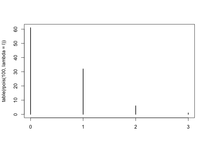
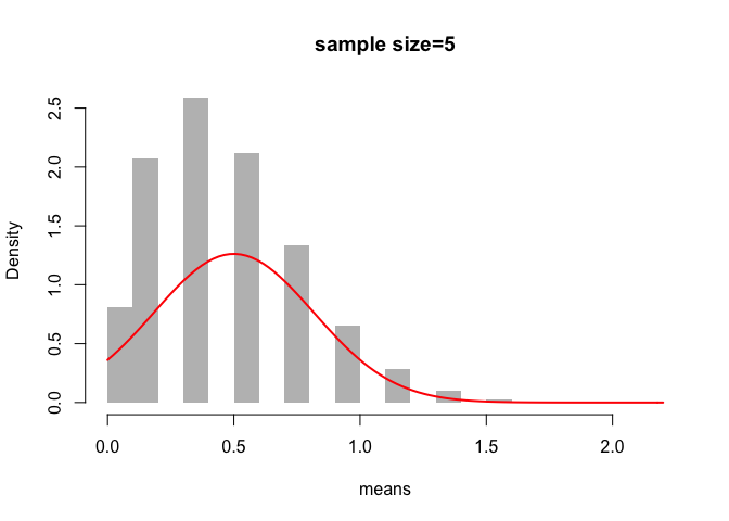
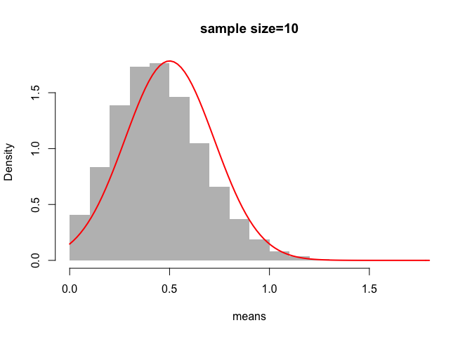
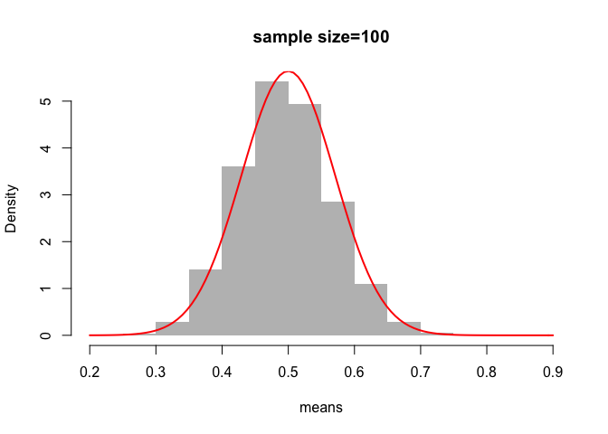
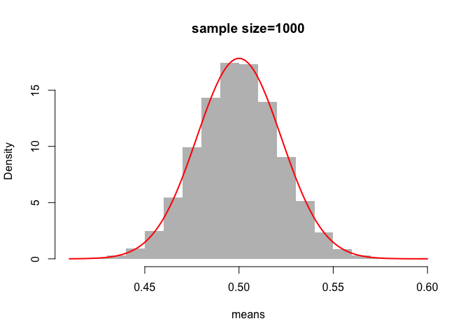
Now for estimating the mean. For each histogram below I have repeated 100000 times the following: draw a sample of $n$ observations from the Poisson with $\lambda=.5$ and estimate $\hat\mu$ in this sample. The histograms thus show 100000 draws from the actual distribution of $\hat \mu$. The red line shows the normal approximation.

At $n=5$ we're not doing so great. Your confidence interval would probably contain some negative values. At $n=10$ it's looking better, but there is still some issue with the truncation at 0. At $n=100$ and $n=1000$ it doesn't look as though we need to worry. This is of course because the distribution gets narrower with larger $n$.

asymptotic_v_actual <- function(sample_size) {
  means <- raply(100000, mean(rpois(sample_size, lambda=l)))
  hist(means, prob=T, col="grey", border = NA,
       main=paste0("sample size=", as.character(sample_size)))
  curve(dnorm(x, mean=l, sd=sqrt(l/sample_size)), add=T, lwd=2, col="red")
}

asymptotic_v_actual(sample_size=5)
asymptotic_v_actual(sample_size=10)
asymptotic_v_actual(sample_size=100)
asymptotic_v_actual(sample_size=1000)
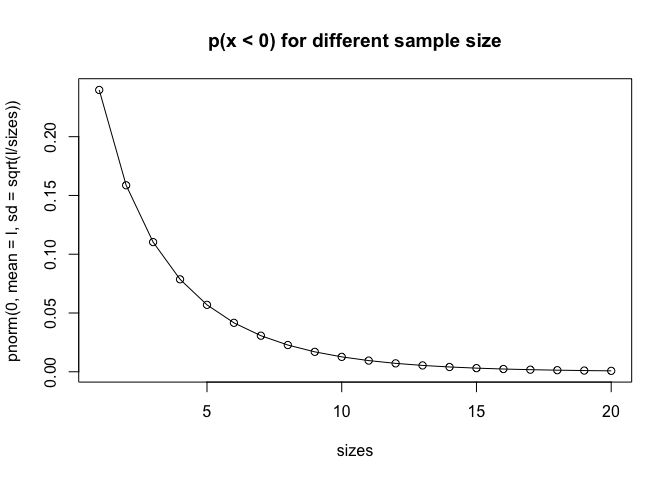
Finally I will show the probability of having $\hat\mu < 0$ according to the normal approximation at different sample sizes. At $n=20$ this is practically zero in our toy example.

# probability of x < 0 for different sample sizes:
sizes <- 1:20
plot(sizes, pnorm(0, mean=l, sd=sqrt(l/sizes)), type="o", 
     main="p(x < 0) for different sample size")

Nonparametric alternative

If you don't want to make any parametric assumptions (if you worry that your data aren't normal enough), you can use the bootstrap to build confidence bands around the estimated mean. This is a computational method that goes roughly as follows (variants exist):

The short answer is yes, you can certainly use these data for inferential statistics.

  You're interested in the mean, so this makes it pretty straight-forward: basically the distribution a mean estimate $\hat \mu$ will converge to a normal distribution with mean $\mu$ (the population mean) and standard deviation $\sigma/\sqrt{n}$. Your underlying data don't have to be normal for this to be true, and can actually look pretty crazy. But the speed of convergence depends on "how normal" the sample is.

Usually $\sigma$ isn't known and you have to estimate it from the data, which leads to some extra uncertainty and the estimate will follow a Student's $t$ distribution. However, at your sample size the normal approximation is probably fine as Student's $t$ is asymptotically normal.

If you don't want to make any parametric assumptions (if you worry that your data aren't normal enough), you can use the bootstrap to build confidence bands. This is a computational method that goes roughly as follows (variants exist):

The short answer is yes, you can certainly use these data for inferential statistics. You're interested in the mean, so this makes it pretty straight-forward.

The usual parametric confidence interval

The distribution of a mean estimate $\hat \mu$ will (per the central limit theorem) converge to a normal distribution with mean $\mu$ (the population mean) and standard deviation $\sigma/\sqrt{n}$. Your underlying data don't have to be normal for this to be true, and can actually look pretty crazy. But the speed of convergence depends on "how normal" the sample is.

Usually $\sigma$ isn't known and you have to estimate it from the data, which leads to some extra uncertainty and the estimate will follow a Student's $t$ distribution. However, at your sample size the normal approximation is probably fine as Student's $t$ is asymptotically normal. Using this information you just estimate the mean and use the parametric distribution to compute confidence intervals in the usual way.


About the "limits" of your data: So your data is limited below at 5000ms due to physical laws. I'm going to show how this might impact the central-limit-theorem-type confidence interval with some R code and some plots.

Below I sample from a Poisson distribution with $\lambda=.5$. This distribution has mean and variance both $=.5$. This distribution has a limit in the same sense as your data: its support is the non-negative integers, so it has no values below 0. Hence we can never estimate a negative mean from this, as you could never estimate a mean below 5000ms in your data.

The asymptotic normal approximation for the mean of an $n$-sized sample in this setting is $\hat \mu \sim N(0.5, \sqrt{\frac{0.5}{n}})$. A normal distribution has the entire real line as support, so there is some chance of negative numbers here. In some sense the normal approximation must be wrong no matter what! We'll see that this problem is more real for smaller sample sizes. The data look like this:


library(plyr)

set.seed(2017-06-08)

l=0.5

# this distribution has mean and variance both = l above
# importantly it never produces values < 0
plot(table(rpois(100, lambda=l)))

Now for estimating the mean. For each histogram below I have repeated 100000 times the following: draw a sample of $n$ observations from the Poisson with $\lambda=.5$ and estimate $\hat\mu$ in this sample. The histograms thus show 100000 draws from the actual distribution of $\hat \mu$. The red line shows the normal approximation.

At $n=5$ we're not doing so great. Your confidence interval would probably contain some negative values. At $n=10$ it's looking better, but there is still some issue with the truncation at 0. At $n=100$ and $n=1000$ it doesn't look as though we need to worry. This is of course because the distribution gets narrower with larger $n$.

asymptotic_v_actual <- function(sample_size) {
  means <- raply(100000, mean(rpois(sample_size, lambda=l)))
  hist(means, prob=T, col="grey", border = NA,
       main=paste0("sample size=", as.character(sample_size)))
  curve(dnorm(x, mean=l, sd=sqrt(l/sample_size)), add=T, lwd=2, col="red")
}

asymptotic_v_actual(sample_size=5)

asymptotic_v_actual(sample_size=10)

asymptotic_v_actual(sample_size=100)

asymptotic_v_actual(sample_size=1000)

Finally I will show the probability of having $\hat\mu < 0$ according to the normal approximation at different sample sizes. At $n=20$ this is practically zero in our toy example.

# probability of x < 0 for different sample sizes:
sizes <- 1:20
plot(sizes, pnorm(0, mean=l, sd=sqrt(l/sizes)), type="o", 
     main="p(x < 0) for different sample size")


Nonparametric alternative

If you don't want to make any parametric assumptions (if you worry that your data aren't normal enough), you can use the bootstrap to build confidence bands around the estimated mean. This is a computational method that goes roughly as follows (variants exist):

Source Link
einar
  • 4.3k
  • 2
  • 25
  • 39

The short answer is yes, you can certainly use these data for inferential statistics.

You're interested in the mean, so this makes it pretty straight-forward: basically the distribution a mean estimate $\hat \mu$ will converge to a normal distribution with mean $\mu$ (the population mean) and standard deviation $\sigma/\sqrt{n}$. Your underlying data don't have to be normal for this to be true, and can actually look pretty crazy. But the speed of convergence depends on "how normal" the sample is.

Usually $\sigma$ isn't known and you have to estimate it from the data, which leads to some extra uncertainty and the estimate will follow a Student's $t$ distribution. However, at your sample size the normal approximation is probably fine as Student's $t$ is asymptotically normal.

If you don't want to make any parametric assumptions (if you worry that your data aren't normal enough), you can use the bootstrap to build confidence bands. This is a computational method that goes roughly as follows (variants exist):

  1. Make $B$ bootstrap samples by resampling from your original sample with replacement.
  2. Estimate the bootstrapped mean $\hat \mu^*_b$ in each of your bootstrap samples. This gives you an empirical distribution of over $\hat \mu$.
  3. Use the quantiles of this distribution as confidence bands. Eg if you want a 95% confidence interval, use the 0.025 quantile as lower limit, the 0.975 quantile as upper limit.

The bootstrap is very general and the bootstrapped statistic doesn't have to be a mean. If you want to look at the median or something else that isn't as simple to work with as the mean there's always the bootstrap.