added 45 characters in body
Source Link
jld
  • 20.8k
  • 2
  • 64
  • 69

For example, let's consider a network with 1 hidden layer of $N$ units and a linear output layer: our cost function is $$ g(\alpha, W) = \sum_i \left(y_i - \alpha_i\sigma(Wx_i)\right)^2 $$ where $x_i \in \mathbb R^p$ and $W \in \mathbb R^{N \times p}$ (and I'm omitting bias terms for simplicity). This is not necessarily convex when viewed as a function of $(\alpha, W)$ (depending on $\sigma$: if a linear activation function is used then this still can be convex). And the deeper our network gets, the less convex things are.

costfunc <- function(u, v, W, a, x, y, afunc) {
  W[1,1] <- u; W[1,2] <- v
  preds <- t(a) %*% afunc(W %*% t(x))
  sum((y - preds)^2)
}

set.seed(1)
n <- 75  # number of  observations
p <- 3   # number of predictors
N <- 1   # number of hidden layersunits


x <- matrix(rnorm(n * p), n, p)
y <- rnorm(n)  # all noise
a <- matrix(rnorm(N), N)
W <- matrix(rnorm(N * p), N, p)

afunc <- function(z) 1 / (1 + exp(-z))  # sigmoid

l = 400  # dim of matrix of cost evaluations
wvals <- seq(-50, 50, length = l)  # where we evaluate costfunc
fmtx <- matrix(0, l, l)
for(i in 1:l) {
  for(j in 1:l) {
    fmtx[i,j] = costfunc(wvals[i], wvals[j], W, a, x, y, afunc)
  }
}

filled.contour(wvals, wvals, fmtx,plot.axes = { contour(wvals, wvals, fmtx, nlevels = 25, 
                                           drawlabels = F, axes = FALSE, 
                                           frame.plot = FALSE, add = TRUE); axis(1); axis(2) },
               main = 'NN loss surface', xlab = expression(paste('W'[11])), ylab = expression(paste('W'[12])))

For example, let's consider a network with 1 hidden layer of $N$ units and a linear output layer: our cost function is $$ g(\alpha, W) = \sum_i \left(y_i - \alpha_i\sigma(Wx_i)\right)^2 $$ where $x_i \in \mathbb R^p$ and $W \in \mathbb R^{N \times p}$. This is not necessarily convex when viewed as a function of $(\alpha, W)$ (depending on $\sigma$: if a linear activation function is used then this still can be convex). And the deeper our network gets, the less convex things are.

costfunc <- function(u, v, W, a, x, y, afunc) {
  W[1,1] <- u; W[1,2] <- v
  preds <- t(a) %*% afunc(W %*% t(x))
  sum((y - preds)^2)
}

set.seed(1)
n <- 75  # number of  observations
p <- 3  # number of predictors
N <- 1  # number of hidden layers


x <- matrix(rnorm(n * p), n, p)
y <- rnorm(n)  # all noise
a <- matrix(rnorm(N), N)
W <- matrix(rnorm(N * p), N, p)

afunc <- function(z) 1 / (1 + exp(-z))  # sigmoid

l = 400  # dim of matrix of cost evaluations
wvals <- seq(-50, 50, length = l)  # where we evaluate costfunc
fmtx <- matrix(0, l, l)
for(i in 1:l) {
  for(j in 1:l) {
    fmtx[i,j] = costfunc(wvals[i], wvals[j], W, a, x, y, afunc)
  }
}

filled.contour(wvals, wvals, fmtx,plot.axes = { contour(wvals, wvals, fmtx, nlevels = 25, 
                                           drawlabels = F, axes = FALSE, 
                                           frame.plot = FALSE, add = TRUE); axis(1); axis(2) },
               main = 'NN loss surface', xlab = expression(paste('W'[11])), ylab = expression(paste('W'[12])))
For example, let's consider a network with 1 hidden layer of $N$ units and a linear output layer: our cost function is $$ g(\alpha, W) = \sum_i \left(y_i - \alpha_i\sigma(Wx_i)\right)^2 $$ where $x_i \in \mathbb R^p$ and $W \in \mathbb R^{N \times p}$ (and I'm omitting bias terms for simplicity). This is not necessarily convex when viewed as a function of $(\alpha, W)$ (depending on $\sigma$: if a linear activation function is used then this still can be convex). And the deeper our network gets, the less convex things are.

costfunc <- function(u, v, W, a, x, y, afunc) {
  W[1,1] <- u; W[1,2] <- v
  preds <- t(a) %*% afunc(W %*% t(x))
  sum((y - preds)^2)
}

set.seed(1)
n <- 75  # number of observations
p <- 3   # number of predictors
N <- 1   # number of hidden units


x <- matrix(rnorm(n * p), n, p)
y <- rnorm(n)  # all noise
a <- matrix(rnorm(N), N)
W <- matrix(rnorm(N * p), N, p)

afunc <- function(z) 1 / (1 + exp(-z))  # sigmoid

l = 400  # dim of matrix of cost evaluations
wvals <- seq(-50, 50, length = l)  # where we evaluate costfunc
fmtx <- matrix(0, l, l)
for(i in 1:l) {
  for(j in 1:l) {
    fmtx[i,j] = costfunc(wvals[i], wvals[j], W, a, x, y, afunc)
  }
}

filled.contour(wvals, wvals, fmtx,plot.axes = { contour(wvals, wvals, fmtx, nlevels = 25, 
                                           drawlabels = F, axes = FALSE, 
                                           frame.plot = FALSE, add = TRUE); axis(1); axis(2) },
               main = 'NN loss surface', xlab = expression(paste('W'[11])), ylab = expression(paste('W'[12])))
added figure code
Source Link
jld
  • 20.8k
  • 2
  • 64
  • 69

Here's the R code that I used to make this figure (although some of the parameters are at slightly different values now than when I made it so they won't be identical):

costfunc <- function(u, v, W, a, x, y, afunc) {
  W[1,1] <- u; W[1,2] <- v
  preds <- t(a) %*% afunc(W %*% t(x))
  sum((y - preds)^2)
}

set.seed(1)
n <- 75  # number of  observations
p <- 3  # number of predictors
N <- 1  # number of hidden layers


x <- matrix(rnorm(n * p), n, p)
y <- rnorm(n)  # all noise
a <- matrix(rnorm(N), N)
W <- matrix(rnorm(N * p), N, p)

afunc <- function(z) 1 / (1 + exp(-z))  # sigmoid

l = 400  # dim of matrix of cost evaluations
wvals <- seq(-50, 50, length = l)  # where we evaluate costfunc
fmtx <- matrix(0, l, l)
for(i in 1:l) {
  for(j in 1:l) {
    fmtx[i,j] = costfunc(wvals[i], wvals[j], W, a, x, y, afunc)
  }
}

filled.contour(wvals, wvals, fmtx,plot.axes = { contour(wvals, wvals, fmtx, nlevels = 25, 
                                           drawlabels = F, axes = FALSE, 
                                           frame.plot = FALSE, add = TRUE); axis(1); axis(2) },
               main = 'NN loss surface', xlab = expression(paste('W'[11])), ylab = expression(paste('W'[12])))
added 73 characters in body
Source Link
jld
  • 20.8k
  • 2
  • 64
  • 69

$\sum_i (y_i- \hat y_i)^2$ is indeed convex in $\hat y_i$. But if $\hat y_i = f(x_i ; \theta)$ it may not be convex in $\theta$, which is the situation with most non-linear models, and we actually care about convexity in $\theta$ because that's what we're optimizing the cost function over.

For example, let's consider a NNnetwork with 1 hidden layer of $N$ units and a linear output layer: $$ \sum_i \left(y_i - \alpha_i\sigma(Wx)\right)^2 $$ is our cost function, is $$ g(\alpha, W) = \sum_i \left(y_i - \alpha_i\sigma(Wx_i)\right)^2 $$ where $x_i \in \mathbb R^p$ and this$W \in \mathbb R^{N \times p}$. This is not necessarily convex when viewed as a function of $(\alpha, W)$ (depending on $\sigma$: if a linear activation function is used then this still willcan be convex).

A really simple example: if we have $N$ hidden layers then we can look at $$ g(\alpha, W) = \sum_i \left(y_i - \alpha_i \sigma\left( Wx_i \right)\right)^2 $$ where $x_i \in \mathbb R^p$ and $W \in \mathbb R^{N \times p}$ And the deeper our network gets, the less convex things are.

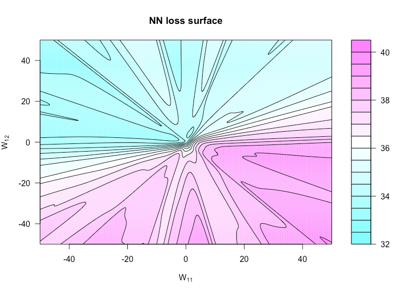
Now define a function $h : \mathbb R \times \mathbb R \to \mathbb R$ by $h(u, v) = g(\alpha, W(u, v))$ where $W(u,v)$ is $W$ with $W_{11}$ set to $u$ and $W_{12}$ set to $v$. This allows us to visualize the cost function as these two weights vary.

The figure below shows this for the sigmoid activation function with $n=50$, $p=3$, and $N=1$ (so an extremely simple architecture). All data (both $x$ and $y$) are iid $\mathcal N(0,1)$, as are any weights not being varied in the plotting function. You can see the lack of convexity here.

loss surface

$\sum_i (y_i- \hat y_i)^2$ is indeed convex in $\hat y_i$. But if $\hat y_i = f(x_i ; \theta)$ it may not be convex in $\theta$, which is the situation with most non-linear models, and we actually care about convexity in $\theta$ because that's what we're optimizing the cost function over.

For example, let's consider a NN with 1 hidden layer: $$ \sum_i \left(y_i - \alpha_i\sigma(Wx)\right)^2 $$ is our cost function, and this is not necessarily convex when viewed as a function of $(\alpha, W)$ (depending on $\sigma$: if a linear activation function is used then this still will be convex).

A really simple example: if we have $N$ hidden layers then we can look at $$ g(\alpha, W) = \sum_i \left(y_i - \alpha_i \sigma\left( Wx_i \right)\right)^2 $$ where $x_i \in \mathbb R^p$ and $W \in \mathbb R^{N \times p}$.

Now define a function $h : \mathbb R \times \mathbb R \to \mathbb R$ by $h(u, v) = g(\alpha, W(u, v))$ where $W(u,v)$ is $W$ with $W_{11}$ set to $u$ and $W_{12}$ set to $v$. This allows us to visualize the cost function as these two weights vary.

The figure below shows this for the sigmoid activation function with $n=50$, $p=3$, and $N=1$ (so an extremely simple architecture). All data (both $x$ and $y$) are iid $\mathcal N(0,1)$, as are any weights not being varied in the plotting function. You can see the lack of convexity here.

loss surface

$\sum_i (y_i- \hat y_i)^2$ is indeed convex in $\hat y_i$. But if $\hat y_i = f(x_i ; \theta)$ it may not be convex in $\theta$, which is the situation with most non-linear models, and we actually care about convexity in $\theta$ because that's what we're optimizing the cost function over.

For example, let's consider a network with 1 hidden layer of $N$ units and a linear output layer: our cost function is $$ g(\alpha, W) = \sum_i \left(y_i - \alpha_i\sigma(Wx_i)\right)^2 $$ where $x_i \in \mathbb R^p$ and $W \in \mathbb R^{N \times p}$. This is not necessarily convex when viewed as a function of $(\alpha, W)$ (depending on $\sigma$: if a linear activation function is used then this still can be convex). And the deeper our network gets, the less convex things are.

Now define a function $h : \mathbb R \times \mathbb R \to \mathbb R$ by $h(u, v) = g(\alpha, W(u, v))$ where $W(u,v)$ is $W$ with $W_{11}$ set to $u$ and $W_{12}$ set to $v$. This allows us to visualize the cost function as these two weights vary.

The figure below shows this for the sigmoid activation function with $n=50$, $p=3$, and $N=1$ (so an extremely simple architecture). All data (both $x$ and $y$) are iid $\mathcal N(0,1)$, as are any weights not being varied in the plotting function. You can see the lack of convexity here.

loss surface

added 73 characters in body
Source Link
jld
  • 20.8k
  • 2
  • 64
  • 69
Loading
Source Link
jld
  • 20.8k
  • 2
  • 64
  • 69
Loading