Think about what a CDF represents in terms of probability. Let the variables on the x-axis be referred to as $x$ and y-axis values be referred to as $y$. By definition the cumulative distribution function is showing the probability that a variable is less than or equal to $x$. More specifically, if you look at $x=0$ for each curve the CDF is telling you: $P_{\text{red}}(X \leq 0) \approx 0.5$ and $P_{\text{green}}(X \leq 0) \approx 0.7$.
Your question is a little vague so I will answer it in two parts.
How meaningful is the difference at a particular point?: Let's assume $X$ represents the difference in points from an average test score (with a negative value representing below average and positive value representing above average). Let the green curve represent boys and red curve represent girls. Now, $P_{\text{red}}(X \leq 0) \approx 0.5$ and $P_{\text{green}}(X \leq 0) \approx 0.7$ tells us that the probability of a boy scoring below average is higher than the probability of a girl scoring below average. If we look at the CDF as whole (green always above red) this suggests in your sample population, girls score higher than boys. Whether or not this result is statistically significant is yet to be determined.
How meaningful is the difference overall? (edited as a response to @whuber) : This depends on how you use it. For instance, if the green CDF represented the CDF of some reference distribution and the red CDF was an empirical sample distribution, then the point by point vertical differences can be used in a Kolmogorov–Smirnov test for equality between the two distributiondistributions.
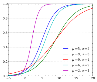
The fact that the green "leads" the red and the two curves are similarly shaped contribute to the fact that the green is always above the red, but this does not necessarily have to be the case. Consider that your populations do not come from the same underlying distribution. In this case the shape of the CDF would differ and the fact that the green "leads" the red would not necessarily result in the green always being above the red. For example, here are various CDFs of a logistic distribution (from Wikipedia)
Notice that the red curve in the plot above "leads" (starts from a nonzero value) before the rest of the curves do, but ultimately end up below most of the curves as the x-values approach x=20.

