###Assumptions and Notation

Let us suppose that the true proportions for the candidates among the actual voters are $p=(p_A,p_B,p_C)$ and that the poll can be viewed as a random sample (without replacement) from all voters. If the poll is a sizable proportion of all voters (more than $10\%$ or so) then we'll need to know the number of voters. Since we don't, let's assume that number is so large that the poll can be analyzed as if it were a random sample with replacement.

###Analysis Under these assumptions the likelihood of observing $a$ votes for $A$, $b$ votes for $B$, and $C$ votes for $c$ is given by the trinomial probability

$$L(p;a,b,c) = \binom{n}{a\,b\,c} p_A^a p_B^b p_C^c$$

with $n=a+b+c$ is the size of the poll.

We may use the theory of Maximum Likelihood to evaluate the possibilities. To this end, as is usual, begin by finding $\hat p$ to maximize $\log L$. Since this function is differentiable, we introduce a Lagrange multiplier $\lambda$ to handle the constraint $g(p)=p_A+p_B+p_C=1$ look for its maximum among its critical points where

$$(0,0,0) = D_p\log (L(p;a,b,c)-\lambda g(p)) =\left(\frac{a}{p_A}-\lambda, \frac{b}{p_B}-\lambda, \frac{c}{p_C}-\lambda\right).$$

The unique solution, which is easily seen to be a local maximum (and therefore the global maximum, since obviously $L$ is not maximal anywhere along the boundary where one or more of the components of $p$ are zero), is

$$\hat p = \left(\frac{a}{n}, \frac{b}{n}, \frac{c}{n}\right).$$

To evaluate the plausibility of any possible value of $p$, compare $\log L(\hat p; a,b,c)$ to $\log L(p;a,b,c)$. When twice the difference exceeds the upper $1-\alpha$ percentile of the $\chi^2(1)$ distribution, we have less than $100\alpha\%$ confidence in such a value of $p$. This is an approximate calculation, but it should give good guidance for a poll this size with such a balanced response.

###Results

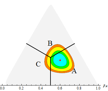
Ordinarily such a result is complicated to interpret, but this situation with just three candidates admits useful visualizations. We may position $p$ on a ternary diagram (which is an orthogonal projection of the simplex $p_A+p_B+p_C=1$ with all $p_i$ nonnegative) and draw the contours of $\log L(\hat p; a,b,c)- \log L(p;a,b,c)$, distinguishing the three regions where $A$, $B$, or $C$ has a majority (that is, where $p_A$ is largest, $p_B$ is largest, and $p_C$ is largest.)

In this ternary diagram, values of $p_A$ plot along the horizontal axis, $p_B$ plots to the up and right, and $p_C$ plots to the left. The value of $\hat p = (45, 30, 25)/100$ is shown as a red dot. The regions corresponding to each of the winners are delineated with the black line segments and labeled accordingly. The red dot, which is safely within $A$'s region, shows $A$ is estimated to be the winner (which is intuitively obvious: $A$ won in this poll).

The contours correspond to confidence levels of $0.92, 0.984, 0.999,$ and $0.9999$, radiating outward from the estimate. The region where $B$ wins is first encountered at the confidence contour of $0.9178$, where $p=(3/8,3/8,1/4)$. This confidence--about $92\%$--is sufficiently far from $100\%$ to suggest $B$ could be the winner, but the corresponding value $\alpha=100-92=8\%$ is small enough to indicate that's a little unlikely. Specifically: if the true proportions were $(3/8,3/8,1/4)$ (or very slightly more for $B$) then $B$ would barely win, but there is some chance--about $100-92 = 8\%$--that this particular poll could have favored $A$ as much as it did, thereby deceiving us.

###Interpretations

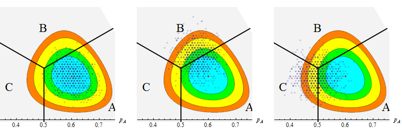
To illustrate this interpretation, I have created three simulations of $1000$ such polls each.

In the first simulation (at the left), the simulation was from a voting population with $p=\hat p = (0.45, 0.30, 0.25)$. Like the poll itself, it obtained $100$ opinions and plotted their proportions here as individual dots. (The dots are partially transparent so that they grow darker where they overlap.) Those $1000$ proportions are scattered around $\hat p$ and lie within the smaller confidence contours, as expected.

For the second simulation the voting population had parameters $p=(3/8,3/8,1/4)$. This on the border between where $A$ and $B$ win, where the $92\%$ contour contacts it. The simulated poll values are of course scattered randomly around it. You can see that several tens, perhaps 50 or more, of the dots favor $A$ even more than the actual poll. This shows why we cannot have high confidence that $B$ will not win.

For the third simulation (at the right) the voting population had parameters $p=(0.35, 0.3, 0.35)$. This is a situation where $C$ can (just barely) win. It's at the $0.984$ contour. This time there are few points that favor $A$ or $B$ as much as the real poll did. This shows why we have little confidence that $C$ will be the winner: there simply are no possible values of $p$ for which a random sample would, by chance, favor $A$ and $B$ over $C$ as much as the actual poll did.

###Discussion

This is a classical interpretation of the maximum likelihood results. It invites you to contemplate possible voting populations, covering the entire ternary diagram, and consider how likely such populations might be to produce poll results like the observed ones. It makes no assumptions about the probabilities of any of these voting populations.

We could proceed further to use this likelihood information to update a prior distribution for the likelihood of winning. This would be an approach akin to those taken by poll aggregators. Unless the prior clearly favors one of the candidates, though, the posterior results should not look much different than shown in the left hand simulation. In simulations using $10^5$ polls with $\hat p$ as the parameter, four percent of the results fall $B$'s winning region and only $0.7$ percent into $C$'s winning region. These numbers could, in a Bayesian interpretation (with a "noninformative prior"), be thought of as the chances that each candidate will win, given the information in the poll and the assumptions that it accurately reflects the voting.