In general, to make your sample mean and variance exactly equal to a pre-specified value, you can appropriately shift and scale the variable. Specifically, if $X_1, X_2, ..., X_n$ is a sample, then the new variables
$$ Z_i = \sqrt{c_{1}} \left( \frac{X_i-\overline{X}}{s_{X}} \right) + c_{2} $$
where $\overline{X} = \frac{1}{n} \sum_{i=1}^{n} X_i$ is the sample mean and $ s^{2}_{X} = \frac{1}{n-1} \sum_{i=1}^{n} (X_i - \overline{X})^2$ is the sample variance are such that the sample mean of the $Z_{i}$'s is exactly $c_2$ and their sample variance is exactly $c_1$. A similarly constructed example can restrict the range -
$$ B_i = a + (b-a) \left( \frac{ X_i - \min (\{X_1, ..., X_n\}) }{\max (\{X_1, ..., X_n\}) - \min (\{X_1, ..., X_n\}) } \right) $$
will produce a data set $B_1, ..., B_n$ that is restricted to the interval $(a,b)$.
Note: These types of shifting/scaling will, in general, change the distributional family of the data, even if the original data comes from a location-scale family.
Within the context of the normal distribution the mvrnorm function in R allows you to simulate normal (or multivariate normal) data with a pre-specified sample mean/covariance by setting empirical=TRUE. Specifically, this function simulates data from the conditional distribution of a normally distributed variable, given the sample mean and (co)variance is equal to a pre-specified value. Note that the resulting marginal distributions are not normal, as pointed out by @whuber in a comment to the main question.
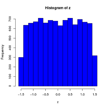
Here is a simple univariate example where the sample mean (from a sample of $n=4$) is constrained to be 0 and the sample standard deviation is 1. We can see that the first element is far more similar to a uniform distribution than a normal distribution:
library(MASS)
 z = rep(0,10000)
for(i in 1:10000)
{
    x = mvrnorm(n = 100004, rep(0,1), 1, tol = 1e-6, empirical = TRUE)
mean(x)
[1] -5.793152e-18
var(x)
   z[i] = [,1]x[1]
[1}
hist(z,]    1col="blue")
$ \ \ \ \ \ \ \ \ \ \ \ \ \ \ \ \ \ $ 
