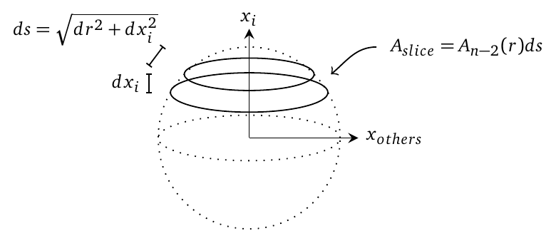
This problem has a very nice geometrical interpretation if we can assume that the distribution $f(\vec{x})$ is constant over the surface of the $n-1$-unit-sphere in $n$-dimensional space. Then $f(\vec{x} \wedge (\vert x_i \vert=a))$ relates to the surface of two slices (at negative and positive coordinate) of the n-1 sphere in n-dimensional space, which is a (n-2)-dimensional sphere with radius $r = \sqrt{1-a^2}$.
The area of this slice is related to the area (or more like a length, since it is a curve) $A_{n-2}$ of the n-2 sphere multiplied with the distance $ds$ which is perpendicular to $\vec{r}$. The fraction of this slice must be related to the total, thus we use the ratio with the area of a $A_{n-1}$ sphere.
We have the area of the slice:
$$A_{slice} = A_{n-2}(r) ds$$
And the relative area of the slice is:
$$\frac{A_{slice}}{A_{total}} = \frac{A_{n-2}(r)}{A_{n-1}(1)} ds$$
with
$$A_{n-2}(r) = \frac{2\pi^{\frac{n-1}{2}}}{\Gamma\left(\frac{n-1}{2}\right)}r^{n-2}$$
$$A_{n-1}(1) = \frac{2\pi^{\frac{n}{2}}}{\Gamma\left(\frac{n}{2}\right)}$$
$$r = \sqrt{1- x_i ^2} $$
$$\begin{array} \\ds &= \sqrt{(dr)^2+(dx_i)^2}\\ %% &= \sqrt{\left(dx_i \frac{-x_i}{\sqrt{1-x_i^2}}\right)^2+(dx_i)^2}\\ %% &= \sqrt{(dx_i)^2 \frac{x_i^2}{{1-x_i^2}}+(dx_i)^2}\\ %% &= \sqrt{(dx_i)^2 \frac{1}{{1-x_i^2}}}\\ &= dx_i {\frac{1}{\sqrt{1-x_i^2}}} \end{array}$$
Thus:
$$\begin{array}\\ f(\vert x_i \vert) &= \frac{2 \Gamma\left(\frac{n}{2}\right)/\Gamma\left(\frac{n-1}{2}\right)}{\pi^{1/2}}\left(1-x_i^2\right)^{\frac{n-3}{2}}\end{array}$$
using the Beta function
$$\begin{array}\\ f(\vert x_i \vert) &= \frac{\left(1-x_i^2\right)^{\frac{n-3}{2}}}{B(\frac{n-1}{2},\frac{1}{2})} \end{array}$$$$\begin{array}\\ f(\vert x_i \vert) &= \frac{\left(1-x_i^2\right)^{\frac{n-3}{2}}}{B(\frac{1}{2},\frac{n-1}{2})} \end{array}$$
which becomes for n=3:
$f(\vert x_i \vert) = 1$
Which makes sense, intuitively. At the pole the slice has smaller radius but is thicker and at the equator the slice has larger radius but is more thin. This results in equal probability, whatever $x_i$ at the pole, the equator, or in between.
Note, some help about the intuition behind the integration step: The n-1 sphere in n-dimensional space is a hypersurface and intersection with $\vert x_i\vert=a$ is a hypercurve. By integrating the hypercurve, along the direction $\vec{s}$, you get the hypersurface

