added 78 characters in body
Source Link
whuber
  • 333.7k
  • 63
  • 792
  • 1.3k

Since data never have lognormal distributions, let's analyze lognormal random variables and then come back to the question of data.

Suppose, then, that $X$ is a random variable with a lognormal distribution. By definition this means $Y=\log(X)$ is almost surely defined and has a Normal$(\mu,\sigma^2)$ distribution for some parameters $\mu$ and $\sigma \gt 0$. In terms of these parameters,

$$E[X] = e^{\mu + \sigma^2/2}$$

and

$$\operatorname{Var}(X) = E[X]^2\left(e^{\sigma^2}-1\right) = e^{2\mu + \sigma^2}\left(e^{\sigma^2}-1\right).$$

(See https://stats.stackexchange.com/a/116657/919 for a derivation.)

We have a great many options to transform $X$ into a new variable $X^\prime$. Among these, the simplest and most natural will correspond to affine transformations of $Y$ to $Y^\prime = \log(X^\prime)$; that is, suppose

$$Y^\prime = a Y + b$$

for some numbers $a$ and $b$, which we proceed to find. In this case the distribution of $Y^\prime$ is still Normal with parameters $$\mu^\prime = a\mu + b$$ and $$(\sigma^\prime)^2 = a^2\sigma^2.$$

Therefore

$$E[X^\prime] = e^{\mu^\prime +(\sigma^\prime)^2/2} = e^{a\mu +b + a^2\sigma^2/2}.$$

Moreover, we want the new variance to be the same as the old, whence

$$e^{2\mu + \sigma^2}\left(e^{\sigma^2}-1\right) = \operatorname{Var}(X) = \operatorname{Var}{X^\prime} = e^{2(a\mu+b) + a^2\sigma^2}\left(e^{a^2\sigma^2}-1\right).$$

Typically there are no solutions (if $E[X^\prime]$ is too small) or two solutions. Writing $m=\log E[X^\prime]$ for the logarithm of the target mean, let

$$d = \log\left(1 - e^{\sigma^2 - 2m + 2\mu} + e^{2\sigma^2 - 2m + 2\mu}\right).$$

Then there is a solution provided $d \ge 0$ and the solution(s) are

$$a = \pm\frac{\sqrt{d}}{\sigma};\quad b = m - \mu a - \frac{d}{2}.$$

Finally, note that the transformation can be expressed directly in terms of $X$ as

$$X^\prime = e^{Y^\prime} = e^{aY + b} = e^{a\log(X)+b} = e^b X^a.$$

It rescales a power of $X$.

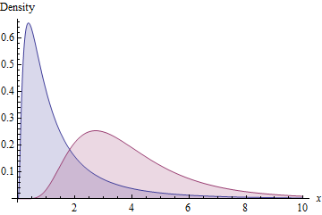
As an illustration, the blue area shows the density function of a Lognormal$(0,1)$ distribution while the red area shows that of a Lognormal distribution with the same standard deviation and mean of $e^m=4$.

Figure

Finally, you might consider applying a comparable transformation to the data: to the extent the data look like they come from a lognormal distribution, this scaled power transformation will produce a new dataset that also looks lognormally distributed with a parent distribution of the same standard deviation. Accordingly, the new data should have almost the same SD as the original data--but, depending on how you estimate the parameters of the parent distribution, the SDs won'tmight not exactly be the same.

Since data never have lognormal distributions, let's analyze lognormal random variables and then come back to the question of data.

Suppose, then, that $X$ is a random variable with a lognormal distribution. By definition this means $Y=\log(X)$ is almost surely defined and has a Normal$(\mu,\sigma^2)$ distribution for some parameters $\mu$ and $\sigma \gt 0$. In terms of these parameters,

$$E[X] = e^{\mu + \sigma^2/2}$$

and

$$\operatorname{Var}(X) = E[X]^2\left(e^{\sigma^2}-1\right) = e^{2\mu + \sigma^2}\left(e^{\sigma^2}-1\right).$$

(See https://stats.stackexchange.com/a/116657/919 for a derivation.)

We have a great many options to transform $X$ into a new variable $X^\prime$. Among these, the simplest and most natural will correspond to affine transformations of $Y$ to $Y^\prime = \log(X^\prime)$; that is, suppose

$$Y^\prime = a Y + b$$

for some numbers $a$ and $b$, which we proceed to find. In this case the distribution of $Y^\prime$ is still Normal with parameters $$\mu^\prime = a\mu + b$$ and $$(\sigma^\prime)^2 = a^2\sigma^2.$$

Therefore

$$E[X^\prime] = e^{\mu^\prime +(\sigma^\prime)^2/2} = e^{a\mu +b + a^2\sigma^2/2}.$$

Moreover, we want the new variance to be the same as the old, whence

$$e^{2\mu + \sigma^2}\left(e^{\sigma^2}-1\right) = \operatorname{Var}(X) = \operatorname{Var}{X^\prime} = e^{2(a\mu+b) + a^2\sigma^2}\left(e^{a^2\sigma^2}-1\right).$$

Typically there are no solutions (if $E[X^\prime]$ is too small) or two solutions. Writing $m=\log E[X^\prime]$ for the logarithm of the target mean, let

$$d = \log\left(1 - e^{\sigma^2 - 2m + 2\mu} + e^{2\sigma^2 - 2m + 2\mu}\right).$$

Then there is a solution provided $d \ge 0$ and the solution(s) are

$$a = \pm\frac{\sqrt{d}}{\sigma};\quad b = m - \mu a - \frac{d}{2}.$$

Finally, note that the transformation can be expressed directly in terms of $X$ as

$$X^\prime = e^{Y^\prime} = e^{aY + b} = e^{a\log(X)+b} = e^b X^a.$$

It rescales a power of $X$.

As an illustration, the blue area shows the density function of a Lognormal$(0,1)$ distribution while the red area shows that of a Lognormal distribution with the same standard deviation and mean of $e^m=4$.

Figure

Finally, you might consider applying a comparable transformation to the data: to the extent the data look like they come from a lognormal distribution, this scaled power transformation will produce a new dataset that also looks lognormally distributed with a parent distribution of the same standard deviation. Accordingly, the new data should have almost the same SD as the original data--but the SDs won't exactly be the same.

Since data never have lognormal distributions, let's analyze lognormal random variables and then come back to the question of data.

Suppose, then, that $X$ is a random variable with a lognormal distribution. By definition this means $Y=\log(X)$ is almost surely defined and has a Normal$(\mu,\sigma^2)$ distribution for some parameters $\mu$ and $\sigma \gt 0$. In terms of these parameters,

$$E[X] = e^{\mu + \sigma^2/2}$$

and

$$\operatorname{Var}(X) = E[X]^2\left(e^{\sigma^2}-1\right) = e^{2\mu + \sigma^2}\left(e^{\sigma^2}-1\right).$$

(See https://stats.stackexchange.com/a/116657/919 for a derivation.)

We have a great many options to transform $X$ into a new variable $X^\prime$. Among these, the simplest and most natural will correspond to affine transformations of $Y$ to $Y^\prime = \log(X^\prime)$; that is, suppose

$$Y^\prime = a Y + b$$

for some numbers $a$ and $b$, which we proceed to find. In this case the distribution of $Y^\prime$ is still Normal with parameters $$\mu^\prime = a\mu + b$$ and $$(\sigma^\prime)^2 = a^2\sigma^2.$$

Therefore

$$E[X^\prime] = e^{\mu^\prime +(\sigma^\prime)^2/2} = e^{a\mu +b + a^2\sigma^2/2}.$$

Moreover, we want the new variance to be the same as the old, whence

$$e^{2\mu + \sigma^2}\left(e^{\sigma^2}-1\right) = \operatorname{Var}(X) = \operatorname{Var}{X^\prime} = e^{2(a\mu+b) + a^2\sigma^2}\left(e^{a^2\sigma^2}-1\right).$$

Typically there are no solutions (if $E[X^\prime]$ is too small) or two solutions. Writing $m=\log E[X^\prime]$ for the logarithm of the target mean, let

$$d = \log\left(1 - e^{\sigma^2 - 2m + 2\mu} + e^{2\sigma^2 - 2m + 2\mu}\right).$$

Then there is a solution provided $d \ge 0$ and the solution(s) are

$$a = \pm\frac{\sqrt{d}}{\sigma};\quad b = m - \mu a - \frac{d}{2}.$$

Finally, note that the transformation can be expressed directly in terms of $X$ as

$$X^\prime = e^{Y^\prime} = e^{aY + b} = e^{a\log(X)+b} = e^b X^a.$$

It rescales a power of $X$.

As an illustration, the blue area shows the density function of a Lognormal$(0,1)$ distribution while the red area shows that of a Lognormal distribution with the same standard deviation and mean of $e^m=4$.

Figure

Finally, you might consider applying a comparable transformation to the data: to the extent the data look like they come from a lognormal distribution, this scaled power transformation will produce a new dataset that also looks lognormally distributed with a parent distribution of the same standard deviation. Accordingly, the new data should have almost the same SD as the original data--but, depending on how you estimate the parameters of the parent distribution, the SDs might not exactly be the same.

Source Link
whuber
  • 333.7k
  • 63
  • 792
  • 1.3k

Since data never have lognormal distributions, let's analyze lognormal random variables and then come back to the question of data.

Suppose, then, that $X$ is a random variable with a lognormal distribution. By definition this means $Y=\log(X)$ is almost surely defined and has a Normal$(\mu,\sigma^2)$ distribution for some parameters $\mu$ and $\sigma \gt 0$. In terms of these parameters,

$$E[X] = e^{\mu + \sigma^2/2}$$

and

$$\operatorname{Var}(X) = E[X]^2\left(e^{\sigma^2}-1\right) = e^{2\mu + \sigma^2}\left(e^{\sigma^2}-1\right).$$

(See https://stats.stackexchange.com/a/116657/919 for a derivation.)

We have a great many options to transform $X$ into a new variable $X^\prime$. Among these, the simplest and most natural will correspond to affine transformations of $Y$ to $Y^\prime = \log(X^\prime)$; that is, suppose

$$Y^\prime = a Y + b$$

for some numbers $a$ and $b$, which we proceed to find. In this case the distribution of $Y^\prime$ is still Normal with parameters $$\mu^\prime = a\mu + b$$ and $$(\sigma^\prime)^2 = a^2\sigma^2.$$

Therefore

$$E[X^\prime] = e^{\mu^\prime +(\sigma^\prime)^2/2} = e^{a\mu +b + a^2\sigma^2/2}.$$

Moreover, we want the new variance to be the same as the old, whence

$$e^{2\mu + \sigma^2}\left(e^{\sigma^2}-1\right) = \operatorname{Var}(X) = \operatorname{Var}{X^\prime} = e^{2(a\mu+b) + a^2\sigma^2}\left(e^{a^2\sigma^2}-1\right).$$

Typically there are no solutions (if $E[X^\prime]$ is too small) or two solutions. Writing $m=\log E[X^\prime]$ for the logarithm of the target mean, let

$$d = \log\left(1 - e^{\sigma^2 - 2m + 2\mu} + e^{2\sigma^2 - 2m + 2\mu}\right).$$

Then there is a solution provided $d \ge 0$ and the solution(s) are

$$a = \pm\frac{\sqrt{d}}{\sigma};\quad b = m - \mu a - \frac{d}{2}.$$

Finally, note that the transformation can be expressed directly in terms of $X$ as

$$X^\prime = e^{Y^\prime} = e^{aY + b} = e^{a\log(X)+b} = e^b X^a.$$

It rescales a power of $X$.

As an illustration, the blue area shows the density function of a Lognormal$(0,1)$ distribution while the red area shows that of a Lognormal distribution with the same standard deviation and mean of $e^m=4$.

Figure

Finally, you might consider applying a comparable transformation to the data: to the extent the data look like they come from a lognormal distribution, this scaled power transformation will produce a new dataset that also looks lognormally distributed with a parent distribution of the same standard deviation. Accordingly, the new data should have almost the same SD as the original data--but the SDs won't exactly be the same.