I find that using direct maximum likelihood with the proper probability function greatly improves estimation of the relative risk. You can directly specify the truncated risk function as the predicted rate for the process.

Usually we use the Hessian to create CIs for the estimate. I have not explored the possibility of using that as the "B" matrix (meat) in the Huber White error and using the fitted risks to get the "A" matrix (bread)... but I suspect it could work! More feasibly you can use a bootstrap to obtain model errors which are robust to a misspecified mean-variance relationship.

## the negative log likelihood for truncated risk function
negLogLik <- function(best, X, y) { 
  pest <- exp(X %*% best)
  -sum(dpois(x = y, lambda = pmin(1, pest), log=TRUE))
}

set.seed(100)

sim <- replicate(100, {
  n <- 200
  X <- cbind(1, 'b'=rbinom(n, 1, 0.5), 'x'=rnorm(n))
  btrue <- c(log(0.3), log(2), 1)
  ptrue <- pmin(1, exp(X %*% matrix(btrue)))
  y <- rbinom(n, 1, ptrue) ## or just take y=ptrue for immediate results
  nlm(f = logLik, p = c(log(mean(y)),0,0), X=X, y=y)$estimate
})

rowMeans(exp(sim))

Gives:

> rowMeans(exp(sim))
[1] 0.3002813 2.0680780 3.0888280

The middle coefficient gives you what you want.

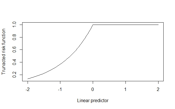
I find that using direct maximum likelihood with the proper probability function greatly improves estimation of the relative risk. You can directly specify the truncated risk function as the predicted rate for the process.

Usually we use the Hessian to create CIs for the estimate. I have not explored the possibility of using that as the "B" matrix (meat) in the Huber White error and using the fitted risks to get the "A" matrix (bread)... but I suspect it could work! More feasibly you can use a bootstrap to obtain model errors which are robust to a misspecified mean-variance relationship.

## the negative log likelihood for truncated risk function
negLogLik <- function(best, X, y) { 
  pest <- pmin(1, exp(X %*% best))
  -sum(dpois(x = y, lambda = pest, log=TRUE))
}

set.seed(100)

sim <- replicate(100, {
  n <- 200
  X <- cbind(1, 'b'=rbinom(n, 1, 0.5), 'x'=rnorm(n))
  btrue <- c(log(0.3), log(2), 1)
  ptrue <- pmin(1, exp(X %*% matrix(btrue)))
  y <- rbinom(n, 1, ptrue) ## or just take y=ptrue for immediate results
  nlm(f = logLik, p = c(log(mean(y)),0,0), X=X, y=y)$estimate
})

rowMeans(exp(sim))

Gives:

> rowMeans(exp(sim))
[1] 0.3002813 2.0680780 3.0888280

The middle coefficient gives you what you want.

I find that using direct maximum likelihood with the proper probability function greatly improves estimation of the relative risk. Usually we use the Hessian to create CIs for the estimate. I have not explored the possibility of using that as the "B" matrix (meat) in the Huber White error and using the fitted risks to get the "A" matrix (bread)... but I suspect it could work!

## the negative log likelihood for truncated risk function
negLogLik <- function(best, X, y) { 
  pest <- exp(X %*% best)
  -sum(dpois(x = y, lambda = pmin(1, pest), log=TRUE))
}

set.seed(100)

sim <- replicate(100, {
  n <- 200
  X <- cbind(1, 'b'=rbinom(n, 1, 0.5), 'x'=rnorm(n))
  btrue <- c(log(0.3), log(2), 1)
  ptrue <- pmin(1, exp(X %*% matrix(btrue)))
  y <- rbinom(n, 1, ptrue) ## or just take y=ptrue for immediate results
  nlm(f = logLik, p = c(log(mean(y)),0,0), X=X, y=y)$estimate
})

rowMeans(exp(sim))

Gives:

> rowMeans(exp(sim))
[1] 0.3002813 2.0680780 3.0888280

The middle coefficient gives you what you want.

I find that using direct maximum likelihood with the proper probability function greatly improves estimation of the relative risk. You can directly specify the truncated risk function as the predicted rate for the process.

Usually we use the Hessian to create CIs for the estimate. I have not explored the possibility of using that as the "B" matrix (meat) in the Huber White error and using the fitted risks to get the "A" matrix (bread)... but I suspect it could work! More feasibly you can use a bootstrap to obtain model errors which are robust to a misspecified mean-variance relationship.

## the negative log likelihood for truncated risk function
negLogLik <- function(best, X, y) { 
  pest <- exp(X %*% best)
  -sum(dpois(x = y, lambda = pmin(1, pest), log=TRUE))
}

set.seed(100)

sim <- replicate(100, {
  n <- 200
  X <- cbind(1, 'b'=rbinom(n, 1, 0.5), 'x'=rnorm(n))
  btrue <- c(log(0.3), log(2), 1)
  ptrue <- pmin(1, exp(X %*% matrix(btrue)))
  y <- rbinom(n, 1, ptrue) ## or just take y=ptrue for immediate results
  nlm(f = logLik, p = c(log(mean(y)),0,0), X=X, y=y)$estimate
})

rowMeans(exp(sim))

Gives:

> rowMeans(exp(sim))
[1] 0.3002813 2.0680780 3.0888280

The middle coefficient gives you what you want.