Here are two examples of binomial model fitting where in the second example with have the independent variable modeled as poly() second order polynomial.

How to interpret these 2 results? Why someone would want to use the poly(2), this would be rather overfitting in the context of logistic regression, right?

I understand that for the linear models lm(y ~ x + I(x^2)) with the second order we would check whether the model fits better to our data, minimize the residuals, but logistic regression has no residuals (error terms). Many thanks.

The poly(,2) depicts completely different picture about survival of M/F across age.

library(vcdExtra)
library(ggplot2)
require(gridExtra)

data(Donner, package="vcdExtra")

head(Donner)

# separate linear fits on age for M/F
g1 <- ggplot(Donner, aes(age, survived, color = sex)) + geom_point(position = position_jitter(height = 0.02, width = 0)) +
   stat_smooth(method = "glm", method.args = list(family = binomial),  formula = y ~ x,  alpha = 0.2, size=2, aes(fill = sex))

# separate quadratics
g2 <- ggplot(Donner, aes(age, survived, color = sex)) + geom_point(position = position_jitter(height = 0.02, width = 0)) +
   stat_smooth(method = "glm", method.args = list(family = binomial),  formula = y ~ poly(x,2), alpha = 0.2, size=2, aes(fill = sex))

grid.arrange(g1, g2, ncol=2)

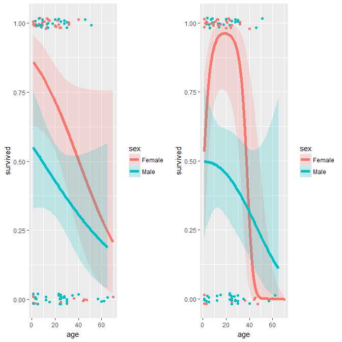
Here are two examples of binomial model fitting. In the second example, the independent variable is modeled using poly() as a second order polynomial.

How do I interpret these 2 results? Why someone would want to use the poly(2)? This would be overfitting in the context of logistic regression, right?

I understand that for the linear models, like lm(y ~ x + I(x^2)), the second order is used to check whether the more complex model provides better fits to our data, vis-a-vis minimizing the residuals, but logistic regression has no residuals (error terms).

The poly(,2) depicts completely different picture about survival of M/F across age.

library(vcdExtra)
library(ggplot2)
require(gridExtra)

data(Donner, package="vcdExtra")

head(Donner)

# separate linear fits on age for M/F
g1 <- ggplot(Donner, aes(age, survived, color = sex)) + geom_point(position = position_jitter(height = 0.02, width = 0)) +
   stat_smooth(method = "glm", method.args = list(family = binomial),  formula = y ~ x,  alpha = 0.2, size=2, aes(fill = sex))

# separate quadratics
g2 <- ggplot(Donner, aes(age, survived, color = sex)) + geom_point(position = position_jitter(height = 0.02, width = 0)) +
   stat_smooth(method = "glm", method.args = list(family = binomial),  formula = y ~ poly(x,2), alpha = 0.2, size=2, aes(fill = sex))

grid.arrange(g1, g2, ncol=2)