Bumped by Community user
added 33 characters in body
Source Link
L.Steele
  • 101
  • 1
  • 1
  • 4

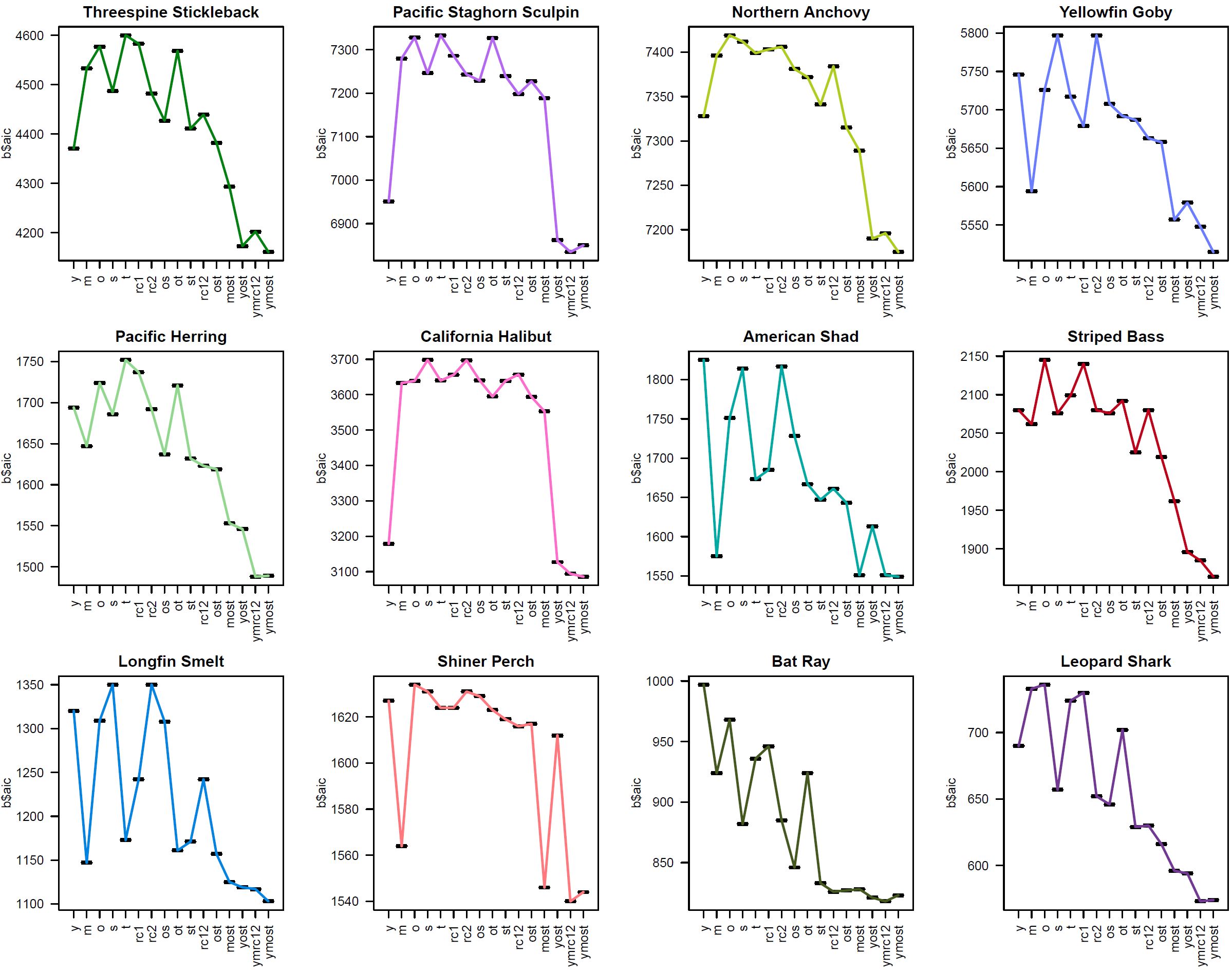
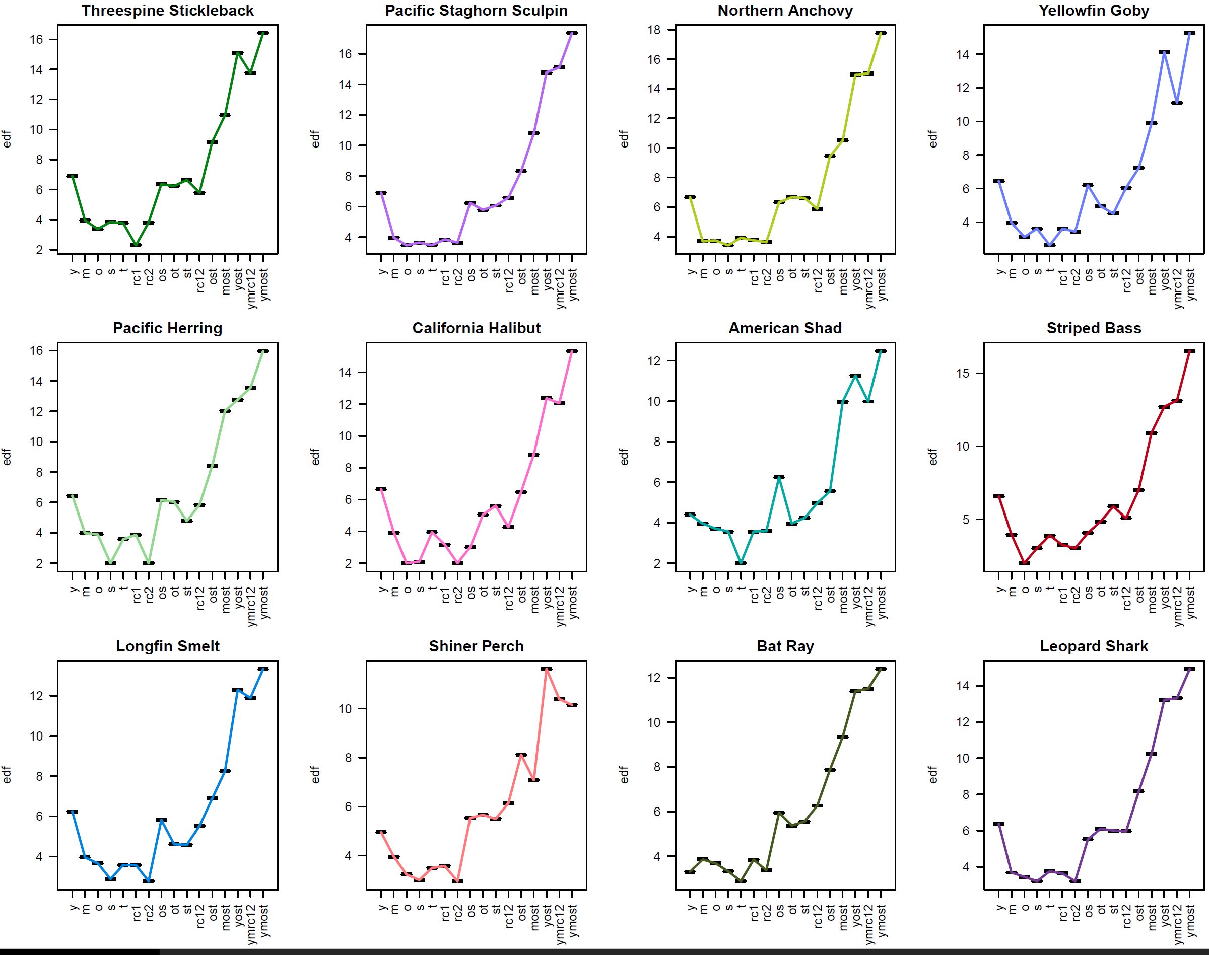
I conducted a bunch of model checks, then plotted the estimated degrees of freedom (edf), deviance explained, edf, and AIC for each model (in order from least to most complex, approximately) to assist with model selection for each species.

EDF EDF

AIC AIC

EDF EDF

I conducted a bunch of model checks, then plotted deviance explained, edf, and AIC for each model (in order from least to most complex, approximately) to assist with model selection for each species.

AIC AIC

EDF EDF

I conducted a bunch of model checks, then plotted the estimated degrees of freedom (edf), deviance explained, and AIC for each model (in order from least to most complex, approximately) to assist with model selection for each species.

EDF EDF

AIC AIC

added 2860 characters in body
Source Link
L.Steele
  • 101
  • 1
  • 1
  • 4

EDF EDF

AIC AIC

EDF EDF

> # GAM based on mtcars 

> library(mgcv)
> b <-gam(mpg~s(hp)+s(wt), data=mtcars)
> summary(b)

Family: gaussian 
Link function: identity 

Formula:
mpg ~ s(hp) + s(wt)

Parametric coefficients:
            Estimate Std. Error t value Pr(>|t|)    
(Intercept)  20.0906     0.3723   53.97   <2e-16 ***
---
Signif. codes:  0 ‘***’ 0.001 ‘**’ 0.01 ‘*’ 0.05 ‘.’ 0.1 ‘ ’ 1

Approximate significance of smooth terms:
        edf Ref.df      F  p-value    
s(hp) 2.409  3.016  6.305  0.00218 ** 
s(wt) 2.085  2.523 15.277 1.19e-05 ***
---
Signif. codes:  0 ‘***’ 0.001 ‘**’ 0.01 ‘*’ 0.05 ‘.’ 0.1 ‘ ’ 1

R-sq.(adj) =  0.878   Deviance explained = 89.6%
GCV = 5.3542  Scale est. = 4.4349    n = 32
> plot(b)
>  


> # logLOG likelihoodLIKELIHOOD ofOF gamGAM modelMODEL (AND DF)

> LL <- logLik(b)
> LL
'log Lik.' -66.22412 (df=6.494385)
>  


> # model degrees ofMODEL freedomDF = no. of parameters (p) = sum of smooth (edf) + parametric (nsdf) terms 

>     # note: intercept gets counted twice (in b$edf and b$nsdf) to attain same df as logLik(b) and aic = AIC(b)
>     # note: summary(b)$pTerms.pv(does not include intercept as a parameter term; gives zero result for unspecified param param)
> p <-  sum(b$edf)+sum(b$nsdf) 
> p
[1] 6.494385
> 
> # AIC = penalty - twice the log likelihood (2p-LL)
> 2*p - 2*LL
'log Lik.' 145.437 (df=6.494385)
> AIC(b)
[1] 145.437
> b$aicb$nsdf) 
> p
[1] 6.494385


> # AIC = penalty - twice the log likelihood (2p-LL)

> 2*p - 2*LL
'log Lik.' 145.437 (df=6.494385)
> AIC(b)
[1] 145.437
> b$aic
[1] 145.437


> #Deviance#DEVIANCE explainedEXPLAINED = 1- (residual dev / total (null) deviance) 

> 1-(b$deviance/b$null.deviance)  
[1] 0.895608
> summary(b)$dev.expl
[1] 0.895608
>
> 
> #Deviance = the unexplained error in the model (residual deviance)
> 2*LL - 2*p    # DOES NOT MATCH b$deviance!$dev.expl
'log[1] Lik0.'895608


> -145.437#DEVIANCE = the unexplained error in the model (df=6.494385residual deviance) 

> b$deviance2*LL - 2*p    # DOES NOT MATCH b$deviance!
'log Lik.' -145.437 (df=6.494385)
> b$deviance
[1] 117.5503
> 

EDF EDF

AIC AIC

> # GAM based on mtcars
> library(mgcv)
> b <-gam(mpg~s(hp)+s(wt), data=mtcars)
> summary(b)

Family: gaussian 
Link function: identity 

Formula:
mpg ~ s(hp) + s(wt)

Parametric coefficients:
            Estimate Std. Error t value Pr(>|t|)    
(Intercept)  20.0906     0.3723   53.97   <2e-16 ***
---
Signif. codes:  0 ‘***’ 0.001 ‘**’ 0.01 ‘*’ 0.05 ‘.’ 0.1 ‘ ’ 1

Approximate significance of smooth terms:
        edf Ref.df      F  p-value    
s(hp) 2.409  3.016  6.305  0.00218 ** 
s(wt) 2.085  2.523 15.277 1.19e-05 ***
---
Signif. codes:  0 ‘***’ 0.001 ‘**’ 0.01 ‘*’ 0.05 ‘.’ 0.1 ‘ ’ 1

R-sq.(adj) =  0.878   Deviance explained = 89.6%
GCV = 5.3542  Scale est. = 4.4349    n = 32
> plot(b)
> 
> # log likelihood of gam model
> LL <- logLik(b)
> LL
'log Lik.' -66.22412 (df=6.494385)
> 
> # model degrees of freedom = no. of parameters (p) = sum of smooth (edf) + parametric (nsdf) terms
>     # note: intercept gets counted twice (in b$edf and b$nsdf) to attain same df as logLik(b) and aic = AIC(b)
>     # note: summary(b)$pTerms.pv(does not include intercept as a parameter term; gives zero result for unspecified param param)
> p <-  sum(b$edf)+sum(b$nsdf) 
> p
[1] 6.494385
> 
> # AIC = penalty - twice the log likelihood (2p-LL)
> 2*p - 2*LL
'log Lik.' 145.437 (df=6.494385)
> AIC(b)
[1] 145.437
> b$aic
[1] 145.437
> 
>
> #Deviance explained = 1- (residual dev / total (null) deviance)
> 1-(b$deviance/b$null.deviance)  
[1] 0.895608
> summary(b)$dev.expl
[1] 0.895608
>
> 
> #Deviance = the unexplained error in the model (residual deviance)
> 2*LL - 2*p    # DOES NOT MATCH b$deviance!
'log Lik.' -145.437 (df=6.494385)
> b$deviance
[1] 117.5503
> 

AIC AIC

EDF EDF

> # GAM based on mtcars 

> library(mgcv)
> b <-gam(mpg~s(hp)+s(wt), data=mtcars)
> summary(b)

Family: gaussian 
Link function: identity 

Formula:
mpg ~ s(hp) + s(wt)

Parametric coefficients:
            Estimate Std. Error t value Pr(>|t|)    
(Intercept)  20.0906     0.3723   53.97   <2e-16 ***
---
Signif. codes:  0 ‘***’ 0.001 ‘**’ 0.01 ‘*’ 0.05 ‘.’ 0.1 ‘ ’ 1

Approximate significance of smooth terms:
        edf Ref.df      F  p-value    
s(hp) 2.409  3.016  6.305  0.00218 ** 
s(wt) 2.085  2.523 15.277 1.19e-05 ***
---
Signif. codes:  0 ‘***’ 0.001 ‘**’ 0.01 ‘*’ 0.05 ‘.’ 0.1 ‘ ’ 1

R-sq.(adj) =  0.878   Deviance explained = 89.6%
GCV = 5.3542  Scale est. = 4.4349    n = 32
> plot(b)


> # LOG LIKELIHOOD OF GAM MODEL (AND DF)

> LL <- logLik(b)
> LL
'log Lik.' -66.22412 (df=6.494385)


> # MODEL DF = no. of parameters (p) = sum of smooth (edf) + parametric (nsdf) terms 

>     # note: intercept gets counted twice (in b$edf and b$nsdf) to attain same df as logLik(b) and aic = AIC(b)
>     # note: summary(b)$pTerms.pv(does not include intercept as a parameter term; gives zero result for unspecified param param)
> p <-  sum(b$edf)+sum(b$nsdf) 
> p
[1] 6.494385


> # AIC = penalty - twice the log likelihood (2p-LL)

> 2*p - 2*LL
'log Lik.' 145.437 (df=6.494385)
> AIC(b)
[1] 145.437
> b$aic
[1] 145.437


> #DEVIANCE EXPLAINED = 1- (residual dev / total (null) deviance) 

> 1-(b$deviance/b$null.deviance)  
[1] 0.895608
> summary(b)$dev.expl
[1] 0.895608


> #DEVIANCE = the unexplained error in the model (residual deviance) 

> 2*LL - 2*p    # DOES NOT MATCH b$deviance!
'log Lik.' -145.437 (df=6.494385)
> b$deviance
[1] 117.5503
> 
added 2860 characters in body
Source Link
L.Steele
  • 101
  • 1
  • 1
  • 4

Here is a simple reproducablereproducible example from mtcars showing the same pattern:

MTCARS GAM Example: AIC vs Dev.Expl & model$aic vs AIC(model) MTCARS GAM Example
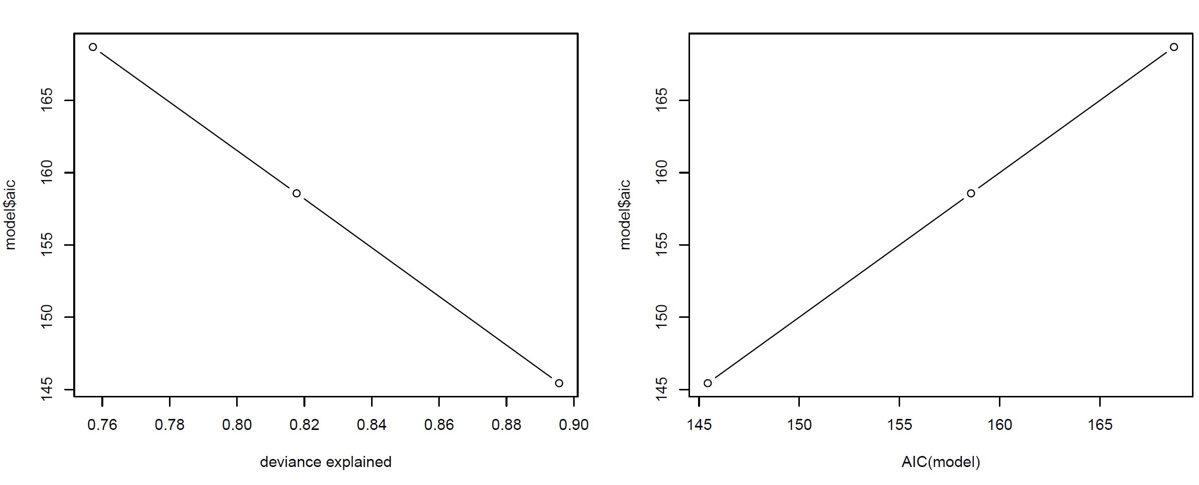
Following the helpful comment by Jon (below), I explored further how gam terms are being calculated in mgcv using the 2-factor gam for mtcars (b3, above). I was able to calculate deviance explained and AIC, which matched model outputs (though calculation of df seemed to double-count the intercept to get the same df as the gam output; odd).

MTCARS GAM SMOOTH mtcars gam smooth
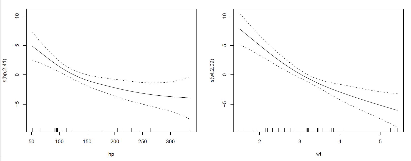
The only calculation I could not get to work was Deviance. The model provided suggests deviance=2logL(model|data)−constant). I, assuming the same constant 2*p as for AIC, could not produce the same result as the gam model output. This only proves that, though grasping AIC and dev.expl, I still don't understand how Deviance is calculated and its relationship to AIC.

> # GAM based on mtcars
> library(mgcv)
> b <-gam(mpg~s(hp)+s(wt), data=mtcars)
> summary(b)

Family: gaussian 
Link function: identity 

Formula:
mpg ~ s(hp) + s(wt)

Parametric coefficients:
            Estimate Std. Error t value Pr(>|t|)    
(Intercept)  20.0906     0.3723   53.97   <2e-16 ***
---
Signif. codes:  0 ‘***’ 0.001 ‘**’ 0.01 ‘*’ 0.05 ‘.’ 0.1 ‘ ’ 1

Approximate significance of smooth terms:
        edf Ref.df      F  p-value    
s(hp) 2.409  3.016  6.305  0.00218 ** 
s(wt) 2.085  2.523 15.277 1.19e-05 ***
---
Signif. codes:  0 ‘***’ 0.001 ‘**’ 0.01 ‘*’ 0.05 ‘.’ 0.1 ‘ ’ 1

R-sq.(adj) =  0.878   Deviance explained = 89.6%
GCV = 5.3542  Scale est. = 4.4349    n = 32
> plot(b)
> 
> # log likelihood of gam model
> LL <- logLik(b)
> LL
'log Lik.' -66.22412 (df=6.494385)
> 
> # model degrees of freedom = no. of parameters (p) = sum of smooth (edf) + parametric (nsdf) terms
>     # note: intercept gets counted twice (in b$edf and b$nsdf) to attain same df as logLik(b) and aic = AIC(b)
>     # note: summary(b)$pTerms.pv(does not include intercept as a parameter term; gives zero result for unspecified param param)
> p <-  sum(b$edf)+sum(b$nsdf) 
> p
[1] 6.494385
> 
> # AIC = penalty - twice the log likelihood (2p-LL)
> 2*p - 2*LL
'log Lik.' 145.437 (df=6.494385)
> AIC(b)
[1] 145.437
> b$aic
[1] 145.437
> 
>
> #Deviance explained = 1- (residual dev / total (null) deviance)
> 1-(b$deviance/b$null.deviance)  
[1] 0.895608
> summary(b)$dev.expl
[1] 0.895608
>
> 
> #Deviance = the unexplained error in the model (residual deviance)
> 2*LL - 2*p    # DOES NOT MATCH b$deviance!
'log Lik.' -145.437 (df=6.494385)
> b$deviance
[1] 117.5503
> 

Any further thoughts would be greatly appreciated.

Here is a simple reproducable example from mtcars showing the same pattern:

MTCARS GAM Example: AIC vs Dev.Expl & model$aic vs AIC(model) MTCARS GAM Example

Here is a simple reproducible example from mtcars showing the same pattern:

MTCARS GAM Example: AIC vs Dev.Expl & model$aic vs AIC(model) MTCARS GAM Example

Following the helpful comment by Jon (below), I explored further how gam terms are being calculated in mgcv using the 2-factor gam for mtcars (b3, above). I was able to calculate deviance explained and AIC, which matched model outputs (though calculation of df seemed to double-count the intercept to get the same df as the gam output; odd).

MTCARS GAM SMOOTH mtcars gam smooth

The only calculation I could not get to work was Deviance. The model provided suggests deviance=2logL(model|data)−constant). I, assuming the same constant 2*p as for AIC, could not produce the same result as the gam model output. This only proves that, though grasping AIC and dev.expl, I still don't understand how Deviance is calculated and its relationship to AIC.

> # GAM based on mtcars
> library(mgcv)
> b <-gam(mpg~s(hp)+s(wt), data=mtcars)
> summary(b)

Family: gaussian 
Link function: identity 

Formula:
mpg ~ s(hp) + s(wt)

Parametric coefficients:
            Estimate Std. Error t value Pr(>|t|)    
(Intercept)  20.0906     0.3723   53.97   <2e-16 ***
---
Signif. codes:  0 ‘***’ 0.001 ‘**’ 0.01 ‘*’ 0.05 ‘.’ 0.1 ‘ ’ 1

Approximate significance of smooth terms:
        edf Ref.df      F  p-value    
s(hp) 2.409  3.016  6.305  0.00218 ** 
s(wt) 2.085  2.523 15.277 1.19e-05 ***
---
Signif. codes:  0 ‘***’ 0.001 ‘**’ 0.01 ‘*’ 0.05 ‘.’ 0.1 ‘ ’ 1

R-sq.(adj) =  0.878   Deviance explained = 89.6%
GCV = 5.3542  Scale est. = 4.4349    n = 32
> plot(b)
> 
> # log likelihood of gam model
> LL <- logLik(b)
> LL
'log Lik.' -66.22412 (df=6.494385)
> 
> # model degrees of freedom = no. of parameters (p) = sum of smooth (edf) + parametric (nsdf) terms
>     # note: intercept gets counted twice (in b$edf and b$nsdf) to attain same df as logLik(b) and aic = AIC(b)
>     # note: summary(b)$pTerms.pv(does not include intercept as a parameter term; gives zero result for unspecified param param)
> p <-  sum(b$edf)+sum(b$nsdf) 
> p
[1] 6.494385
> 
> # AIC = penalty - twice the log likelihood (2p-LL)
> 2*p - 2*LL
'log Lik.' 145.437 (df=6.494385)
> AIC(b)
[1] 145.437
> b$aic
[1] 145.437
> 
>
> #Deviance explained = 1- (residual dev / total (null) deviance)
> 1-(b$deviance/b$null.deviance)  
[1] 0.895608
> summary(b)$dev.expl
[1] 0.895608
>
> 
> #Deviance = the unexplained error in the model (residual deviance)
> 2*LL - 2*p    # DOES NOT MATCH b$deviance!
'log Lik.' -145.437 (df=6.494385)
> b$deviance
[1] 117.5503
> 

Any further thoughts would be greatly appreciated.
Source Link
L.Steele
  • 101
  • 1
  • 1
  • 4
Loading