Bounty Ended with 25 reputation awarded by CommunityBot
about tests
Source Link
David Dale
  • 2.3k
  • 11
  • 19

The distribution of word frequencies is often characterized by Zipf's law, which states that it has Pareto distribution $p(k) \sim k^{-s}$, so-called power law.

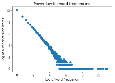
This power law can be well seen as a straight line on the log-log plot of word counts:

import nltk.corpus
import numpy as np
import matplotlib.pyplot as plt
from collections import Counter
# may need nltk.download() to use Brown corpus
counter_of_words = Counter(nltk.corpus.brown.words())
counter_of_counts = Counter(counter_of_words.values())
word_counts = np.array(list(counter_of_counts.keys()))
freq_of_word_counts = np.array(list(counter_of_counts.values()))
plt.scatter(np.log(word_counts), np.log(freq_of_word_counts))
plt.xlabel('Log of word frequency')
plt.ylabel('Log of number of such words')
plt.title('Power law for word frequencies')
plt.show();

enter image description here

The negated slope of this line (roughly -00.5) corresponds to the parameter $s$ of the Zipf law. You can estimate this value with maximizing likelihood:

def neg_zipf_likelihood(s):
    n = sum(freq_of_word_counts)
    # for each word count, find the probability that a random word has such word count
    probas = word_counts ** (-s) / np.sum(np.arange(1, n+1) **(-s))
    log_likelihood = sum(np.log(probas) * word_counts)
    return -log_likelihood

from scipy.optimize import minimize_scalar
s_best = minimize_scalar(neg_zipf_likelihood, [0.1, 3.0] )
print(s_best.x)

which gives you the value of 0.5366.

If you are still not sure whether you need Zipf's distribution or any other distribution, you can compare log likelihood of your data under different distribution, or choose one using Kolmogorov-Smirnov test.

The distribution of word frequencies is often characterized by Zipf's law, which states that it has Pareto distribution $p(k) \sim k^{-s}$, so-called power law.

This power law can be well seen as a straight line on the log-log plot of word counts:

import nltk.corpus
import numpy as np
import matplotlib.pyplot as plt
from collections import Counter
# may need nltk.download() to use Brown corpus
counter_of_words = Counter(nltk.corpus.brown.words())
counter_of_counts = Counter(counter_of_words.values())
word_counts = np.array(list(counter_of_counts.keys()))
freq_of_word_counts = np.array(list(counter_of_counts.values()))
plt.scatter(np.log(word_counts), np.log(freq_of_word_counts))
plt.xlabel('Log of word frequency')
plt.ylabel('Log of number of such words')
plt.title('Power law for word frequencies')
plt.show();

enter image description here

The slope of this line (roughly -0.5) corresponds to the parameter $s$ of the Zipf law. You can estimate this value with maximizing likelihood:

def neg_zipf_likelihood(s):
    n = sum(freq_of_word_counts)
    # for each word count, find the probability that a random word has such word count
    probas = word_counts ** (-s) / np.sum(np.arange(1, n+1) **(-s))
    log_likelihood = sum(np.log(probas) * word_counts)
    return -log_likelihood

from scipy.optimize import minimize_scalar
s_best = minimize_scalar(neg_zipf_likelihood, [0.1, 3.0] )
print(s_best.x)

which gives you the value of 0.5366.

The distribution of word frequencies is often characterized by Zipf's law, which states that it has Pareto distribution $p(k) \sim k^{-s}$, so-called power law.

This power law can be well seen as a straight line on the log-log plot of word counts:

import nltk.corpus
import numpy as np
import matplotlib.pyplot as plt
from collections import Counter
# may need nltk.download() to use Brown corpus
counter_of_words = Counter(nltk.corpus.brown.words())
counter_of_counts = Counter(counter_of_words.values())
word_counts = np.array(list(counter_of_counts.keys()))
freq_of_word_counts = np.array(list(counter_of_counts.values()))
plt.scatter(np.log(word_counts), np.log(freq_of_word_counts))
plt.xlabel('Log of word frequency')
plt.ylabel('Log of number of such words')
plt.title('Power law for word frequencies')
plt.show();

enter image description here

The negated slope of this line (roughly 0.5) corresponds to the parameter $s$ of the Zipf law. You can estimate this value with maximizing likelihood:

def neg_zipf_likelihood(s):
    n = sum(freq_of_word_counts)
    # for each word count, find the probability that a random word has such word count
    probas = word_counts ** (-s) / np.sum(np.arange(1, n+1) **(-s))
    log_likelihood = sum(np.log(probas) * word_counts)
    return -log_likelihood

from scipy.optimize import minimize_scalar
s_best = minimize_scalar(neg_zipf_likelihood, [0.1, 3.0] )
print(s_best.x)

which gives you the value of 0.5366.

If you are still not sure whether you need Zipf's distribution or any other distribution, you can compare log likelihood of your data under different distribution, or choose one using Kolmogorov-Smirnov test.

Source Link
David Dale
  • 2.3k
  • 11
  • 19

The distribution of word frequencies is often characterized by Zipf's law, which states that it has Pareto distribution $p(k) \sim k^{-s}$, so-called power law.

This power law can be well seen as a straight line on the log-log plot of word counts:

import nltk.corpus
import numpy as np
import matplotlib.pyplot as plt
from collections import Counter
# may need nltk.download() to use Brown corpus
counter_of_words = Counter(nltk.corpus.brown.words())
counter_of_counts = Counter(counter_of_words.values())
word_counts = np.array(list(counter_of_counts.keys()))
freq_of_word_counts = np.array(list(counter_of_counts.values()))
plt.scatter(np.log(word_counts), np.log(freq_of_word_counts))
plt.xlabel('Log of word frequency')
plt.ylabel('Log of number of such words')
plt.title('Power law for word frequencies')
plt.show();

enter image description here

The slope of this line (roughly -0.5) corresponds to the parameter $s$ of the Zipf law. You can estimate this value with maximizing likelihood:

def neg_zipf_likelihood(s):
    n = sum(freq_of_word_counts)
    # for each word count, find the probability that a random word has such word count
    probas = word_counts ** (-s) / np.sum(np.arange(1, n+1) **(-s))
    log_likelihood = sum(np.log(probas) * word_counts)
    return -log_likelihood

from scipy.optimize import minimize_scalar
s_best = minimize_scalar(neg_zipf_likelihood, [0.1, 3.0] )
print(s_best.x)

which gives you the value of 0.5366.