added 284 characters in body
Source Link
AdamO
  • 64.8k
  • 6
  • 134
  • 273

The probability

$$P(\text{Not reject }\mathcal{H}_0 \text{ given } |p - 0.5| \ge 0.1) \le 0.05$$

Is the type II error rate. In this case, 1 minus that probability is the power. Therefore, it is a sample size calculation to achieve a power of 0.95 or greater with an effect of $p \ge 0.6$ or $p \le 0.4$.

The 0.1 is not a margin of error. A margin of error applies to an estimate. However, you are referring to the truth (data generating mechanism) which has no margin of error (it isn't random). To calculate the minimum sample size, you have to choose the most conservative value, which as stated is 0.6 (or 0.4 which is WLOG equivalent).

This is nice, because formulated thusly, we can use off-the-shelf power calculators to calculate minimal sample size to achieve a desired power. The pwr package uses the 1988 Cohen transformation for a one-sample test. We can also check with simulation:

pwr.p.test(h=ES.h(0.5,0.6), sig.level=0.05, power=0.95)

gives:

 proportion power calculation for binomial distribution (arcsine transformation) 

          h = 0.2013579
          n = 320.5008
  sig.level = 0.05
      power = 0.95
alternative = two.sided

Which is much more conservative than your n=500 finding. Checking with simulation:

set.seed(123)
n <- 320
p <- 0.6
SIMS <- rbinom(10000, n, p)
SIMS <- cbind(SIMS, n-SIMS)
SIMS <- apply(SIMS, 1, function(x) chisq.test(x)$p.value)
mean(SIMS < 0.05)

gives

> mean(SIMS < 0.05)
[1] 0.9499

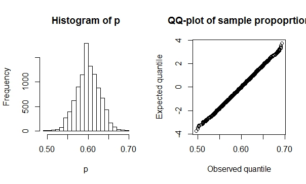
Which is as stated. The important thing is that with $N=300$ (or even much smaller), the asymptotic sampling distribution of the sample mean is very close to normal. Using our SIMS data from above, you can see:

enter image description here

The probability

$$P(\text{Not reject }\mathcal{H}_0 \text{ given } |p - 0.5| \ge 0.1) \le 0.05$$

Is the type II error rate. In this case, 1 minus that probability is the power. Therefore, it is a sample size calculation to achieve a power of 0.95 or greater with an effect of $p \ge 0.6$ or $p \le 0.4$.

The 0.1 is not a margin of error. A margin of error applies to an estimate. However, you are referring to the truth (data generating mechanism) which has no margin of error (it isn't random). To calculate the minimum sample size, you have to choose the most conservative value, which as stated is 0.6 (or 0.4 which is WLOG equivalent).

This is nice, because formulated thusly, we can use off-the-shelf power calculators to calculate minimal sample size to achieve a desired power. The pwr package uses the 1988 Cohen transformation for a one-sample test. We can also check with simulation:

pwr.p.test(h=ES.h(0.5,0.6), sig.level=0.05, power=0.95)

gives:

 proportion power calculation for binomial distribution (arcsine transformation) 

          h = 0.2013579
          n = 320.5008
  sig.level = 0.05
      power = 0.95
alternative = two.sided

Which is much more conservative than your n=500 finding. Checking with simulation:

set.seed(123)
n <- 320
p <- 0.6
SIMS <- rbinom(10000, n, p)
SIMS <- cbind(SIMS, n-SIMS)
SIMS <- apply(SIMS, 1, function(x) chisq.test(x)$p.value)
mean(SIMS < 0.05)

gives

> mean(SIMS < 0.05)
[1] 0.9499

Which is as stated.

The probability

$$P(\text{Not reject }\mathcal{H}_0 \text{ given } |p - 0.5| \ge 0.1) \le 0.05$$

Is the type II error rate. In this case, 1 minus that probability is the power. Therefore, it is a sample size calculation to achieve a power of 0.95 or greater with an effect of $p \ge 0.6$ or $p \le 0.4$.

The 0.1 is not a margin of error. A margin of error applies to an estimate. However, you are referring to the truth (data generating mechanism) which has no margin of error (it isn't random). To calculate the minimum sample size, you have to choose the most conservative value, which as stated is 0.6 (or 0.4 which is WLOG equivalent).

This is nice, because formulated thusly, we can use off-the-shelf power calculators to calculate minimal sample size to achieve a desired power. The pwr package uses the 1988 Cohen transformation for a one-sample test. We can also check with simulation:

pwr.p.test(h=ES.h(0.5,0.6), sig.level=0.05, power=0.95)

gives:

 proportion power calculation for binomial distribution (arcsine transformation) 

          h = 0.2013579
          n = 320.5008
  sig.level = 0.05
      power = 0.95
alternative = two.sided

Which is much more conservative than your n=500 finding. Checking with simulation:

set.seed(123)
n <- 320
p <- 0.6
SIMS <- rbinom(10000, n, p)
SIMS <- cbind(SIMS, n-SIMS)
SIMS <- apply(SIMS, 1, function(x) chisq.test(x)$p.value)
mean(SIMS < 0.05)

gives

> mean(SIMS < 0.05)
[1] 0.9499

Which is as stated. The important thing is that with $N=300$ (or even much smaller), the asymptotic sampling distribution of the sample mean is very close to normal. Using our SIMS data from above, you can see:

enter image description here

Source Link
AdamO
  • 64.8k
  • 6
  • 134
  • 273

The probability

$$P(\text{Not reject }\mathcal{H}_0 \text{ given } |p - 0.5| \ge 0.1) \le 0.05$$

Is the type II error rate. In this case, 1 minus that probability is the power. Therefore, it is a sample size calculation to achieve a power of 0.95 or greater with an effect of $p \ge 0.6$ or $p \le 0.4$.

The 0.1 is not a margin of error. A margin of error applies to an estimate. However, you are referring to the truth (data generating mechanism) which has no margin of error (it isn't random). To calculate the minimum sample size, you have to choose the most conservative value, which as stated is 0.6 (or 0.4 which is WLOG equivalent).

This is nice, because formulated thusly, we can use off-the-shelf power calculators to calculate minimal sample size to achieve a desired power. The pwr package uses the 1988 Cohen transformation for a one-sample test. We can also check with simulation:

pwr.p.test(h=ES.h(0.5,0.6), sig.level=0.05, power=0.95)

gives:

 proportion power calculation for binomial distribution (arcsine transformation) 

          h = 0.2013579
          n = 320.5008
  sig.level = 0.05
      power = 0.95
alternative = two.sided

Which is much more conservative than your n=500 finding. Checking with simulation:

set.seed(123)
n <- 320
p <- 0.6
SIMS <- rbinom(10000, n, p)
SIMS <- cbind(SIMS, n-SIMS)
SIMS <- apply(SIMS, 1, function(x) chisq.test(x)$p.value)
mean(SIMS < 0.05)

gives

> mean(SIMS < 0.05)
[1] 0.9499

Which is as stated.