added 279 characters in body
Source Link
dimitriy
  • 38.3k
  • 7
  • 84
  • 168

As you can see from comparing the SD between women and within women, the hours worked vary almost as much within each woman as across them (7.5 versus 7.8).

This says that about half of the variation in the data is within women, which is what we saw above. WorkingHere $u$ is the fixed effect, which is average hours seem pretty unpredictableworked by each woman, so sigma_u is the same as the within SD above, and $e$ is the residual. $rho$ is the ratio of SD of u squared over the sum of the squared SDs, or total variance:

You can then bootstrap this ratio:$$ \rho = \frac{\sigma_{u}^2}{\sigma_u^2 + \sigma_e^2} $$

You can then bootstrap the $\rho$ ratio:

This gives you:   

enter image description here

As you can see from comparing the SD between women and within women, the hours worked vary almost as much within each woman as across them.

This says that about half of the variation in the data is within women, which is what we saw above. Working hours seem pretty unpredictable.

You can then bootstrap this ratio:

This gives you:  enter image description here

As you can see from comparing the SD between women and within women, the hours worked vary almost as much within each woman as across them (7.5 versus 7.8).

This says that about half of the variation in the data is within women, which is what we saw above. Here $u$ is the fixed effect, which is average hours worked by each woman, so sigma_u is the same as the within SD above, and $e$ is the residual. $rho$ is the ratio of SD of u squared over the sum of the squared SDs, or total variance:

$$ \rho = \frac{\sigma_{u}^2}{\sigma_u^2 + \sigma_e^2} $$

You can then bootstrap the $\rho$ ratio:

This gives you: 

enter image description here

added 10 characters in body
Source Link
dimitriy
  • 38.3k
  • 7
  • 84
  • 168

You can use some of the panel data commands like xtsum and xtreg, fe to do this. This will give you a couple numbers or their ratio, so this does not quite make for a very interesting graph. One ideaapproach would be to bootstrap the ratio and plot a histogram. I show how to do all this below.

You can use some of the panel data commands like xtsum and xtreg, fe to do this. This will give you a couple numbers or their ratio, so this does not make for a very interesting graph. One idea would be to bootstrap the ratio and plot a histogram. I show how to do all this below.

You can use some of the panel data commands like xtsum and xtreg, fe to do this. This will give you a couple numbers or their ratio, so this does not quite make for a very interesting graph. One approach would be to bootstrap the ratio and plot a histogram. I show how to do all this below.

Source Link
dimitriy
  • 38.3k
  • 7
  • 84
  • 168

You can use some of the panel data commands like xtsum and xtreg, fe to do this. This will give you a couple numbers or their ratio, so this does not make for a very interesting graph. One idea would be to bootstrap the ratio and plot a histogram. I show how to do all this below.

. webuse nlswork, clear
(National Longitudinal Survey.  Young Women 14-26 years of age in 1968)

. xtsum hours

Variable         |      Mean   Std. Dev.       Min        Max |    Observations
-----------------+--------------------------------------------+----------------
hours    overall |  36.55956   9.869623          1        168 |     N =   28467
         between |             7.846585          1       83.5 |     n =    4710
         within  |             7.520712  -2.154726   130.0596 | T-bar = 6.04395

As you can see from comparing the SD between women and within women, the hours worked vary almost as much within each woman as across them.

You can also calculate the ratio using a fixed-effects regression:

. xtreg hours, i(idcode) fe

Fixed-effects (within) regression               Number of obs     =     28,467
Group variable: idcode                          Number of groups  =      4,710

R-sq:                                           Obs per group:
     within  = 0.0000                                         min =          1
     between = 0.0030                                         avg =        6.0
     overall =      .                                         max =         15

                                                F(0,23757)        =       0.00
corr(u_i, Xb)  =      .                         Prob > F          =          .

------------------------------------------------------------------------------
       hours |      Coef.   Std. Err.      t    P>|t|     [95% Conf. Interval]
-------------+----------------------------------------------------------------
       _cons |   36.55956   .0487928   749.28   0.000     36.46392     36.6552
-------------+----------------------------------------------------------------
     sigma_u |  7.8465853
     sigma_e |  8.2323986
         rho |  .47601892   (fraction of variance due to u_i)
------------------------------------------------------------------------------
F test that all u_i=0: F(4709, 23757) = 3.64                 Prob > F = 0.0000

This says that about half of the variation in the data is within women, which is what we saw above. Working hours seem pretty unpredictable.

You can then bootstrap this ratio:

. bootstrap ratio = e(rho), rep(500) seed(123) strata(idcode) saving("rhos.dta", replace): xtreg hours, i(idcode) fe
(running xtreg on estimation sample)
(note: file rhos.dta not found)

Bootstrap replications (500)
----+--- 1 ---+--- 2 ---+--- 3 ---+--- 4 ---+--- 5 
..................................................    50
..................................................   100
..................................................   150
..................................................   200
..................................................   250
..................................................   300
..................................................   350
..................................................   400
..................................................   450
..................................................   500

Bootstrap results

Number of strata   =     4,710                  Number of obs     =     28,467
                                                Replications      =        500

      command:  xtreg hours, i(idcode) fe
        ratio:  e(rho)

------------------------------------------------------------------------------
             |   Observed   Bootstrap                         Normal-based
             |      Coef.   Std. Err.      z    P>|z|     [95% Conf. Interval]
-------------+----------------------------------------------------------------
       ratio |   .4760189    .005062    94.04   0.000     .4660976    .4859402
------------------------------------------------------------------------------

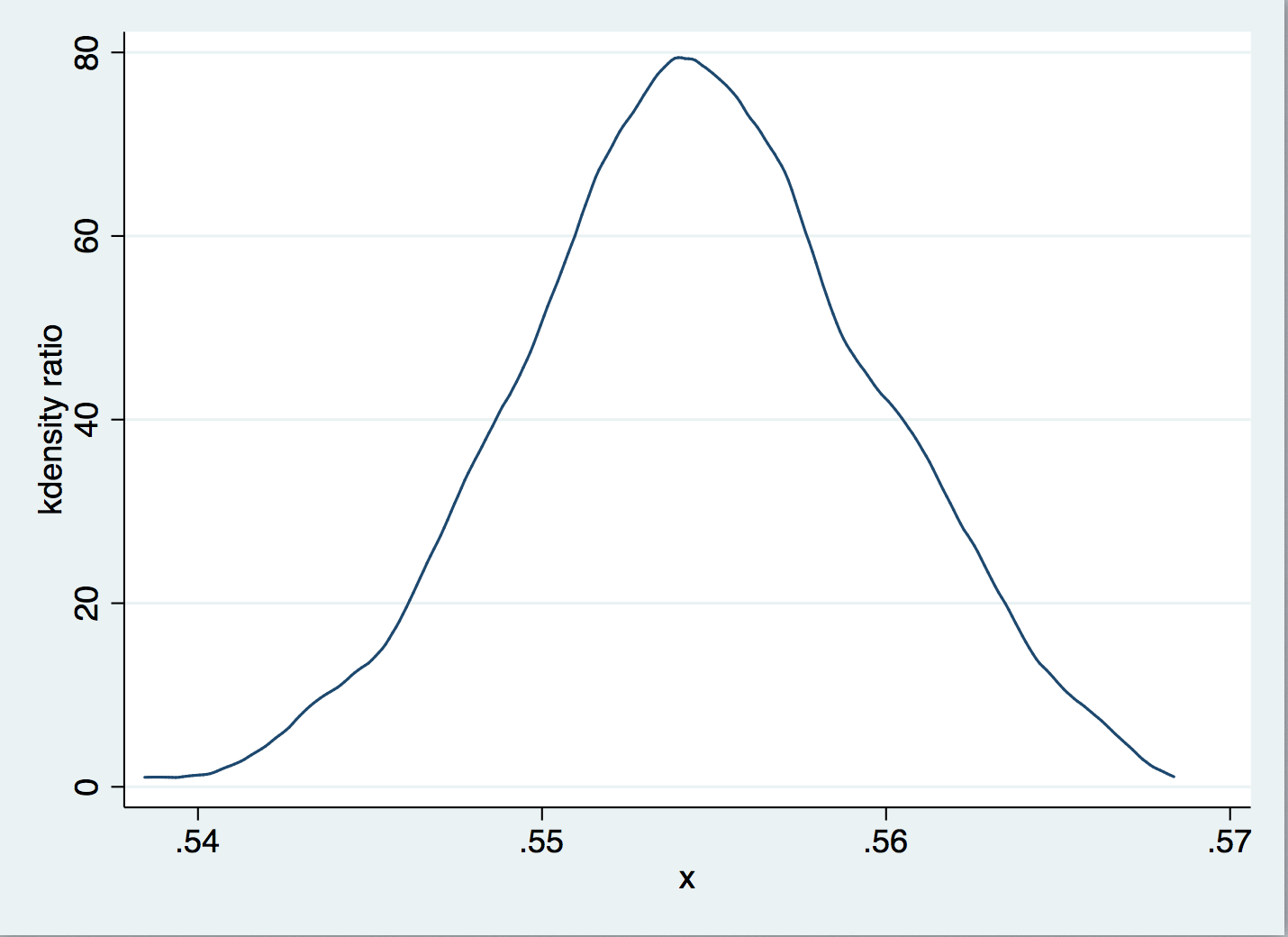
The CI is pretty tight. You can also plot a histogram:

. use "rhos.dta", clear
(bootstrap: xtreg)

. tw kdensity ratio

This gives you: enter image description here