Gaussian process regression (GPR) gives a posterior distribution over functions mapping input to output. We can differentiate to obtain a distribution over the gradient. Below, I'll derive an expression for the expected gradient. There's no need to use finite differencing, as it can be computed in closed form (as long as the covariance function is differentiable; otherwise it doesn't exist).

Expression for the expected gradient

Assume the model:

$$y = f(\mathbf{x}) + \epsilon, \quad \epsilon \underset{\text{i.i.d.}}{\sim} \mathcal{N}(0, \sigma_n^2)$$

where the observed output $y \in \mathbb{R}$ is a function of input $\mathbf{x} \in \mathbb{R}^d$, plus i.i.d. Gaussian noise with variance $\sigma_n^2$. Say we fit a GPR model with differentiable covariance function $k$. Let $X = \{\mathbf{x_1}, \dots, \mathbf{x_n}\}$ denote the training inputs, and let $\mathbf{y} = [y_1, \dots, y_n]^T$ denote the corresponding training outputs. Let $\mathbf{x_*}$ denote a new input, and let $f_*$ be a random variable representing the function value at $\mathbf{x_*}$.

We want to compute $E[\nabla f_* \mid X, \mathbf{y}, \mathbf{x^*}]$, the expected gradient of the function evaluated at $\mathbf{x_*}$ (where the gradient is taken w.r.t. the input and the expectation is over the GPR posterior distribution). Because differentiation is a linear operation, this is equivalent to $\nabla E[ f_* \mid X, \mathbf{y}, \mathbf{x_*}]$, the gradient of the expected function value (i.e. posterior mean) at $\mathbf{x_*}$.

The expected function value at $\mathbf{x_*}$ is:

$$E[f_* \mid X, \mathbf{y}, \mathbf{x_*}] = \sum_{i=1}^n \alpha_i k(\mathbf{x_i}, \mathbf{x_*})$$

where $\mathbf{\alpha} = (K + \sigma_n^2 I)^{-1} \mathbf{y}$, $I$ is the identity matrix, and matrix $K$ contains the covariance for all pairs of training points ($K_{ij} = k(\mathbf{x_i}, \mathbf{x_j})$). For details, see chapter 2 of Rasmussen and Williams (2006).

Taking the gradient, we have:

$$\nabla E[f_* \mid X, \mathbf{y}, \mathbf{x_*}] = \nabla \sum_{i=1}^n \alpha_i \nabla k(\mathbf{x_*}, \mathbf{x_i})$$$$\nabla E[f_* \mid X, \mathbf{y}, \mathbf{x_*}] = \nabla \sum_{i=1}^n \alpha_i k(\mathbf{x_*}, \mathbf{x_i})$$

$$= \sum_{i=1}^n \alpha_i \nabla k(\mathbf{x_*}, \mathbf{x_i})$$

Note that the weights $\mathbf{\alpha}$ are the same as used to compute the expected function value at $\mathbf{x^*}$. So, to compute the expected gradient, the only extra thing we need is the gradient of the covariance function.

For the squared exponential covariance function

As an example, the squared exponential (a.k.a. RBF) covariance function with signal variance $\sigma_f^2$ and length-scale $\ell$ is:

$$k(\mathbf{x}, \mathbf{x'}) = \sigma_f^2 \exp \left[ -\frac{\|\mathbf{x}-\mathbf{x'}\|^2}{2\ell^2} \right]$$

Taking $k(\mathbf{x_*}, \mathbf{x_i})$ and differentiating w.r.t. $\mathbf{x_*}$ gives:

$$\nabla k(\mathbf{x_*}, \mathbf{x_i}) = k(\mathbf{x_*}, \mathbf{x_i}) \frac{\mathbf{x_i} - \mathbf{x_*}}{\ell^2}$$

This can be plugged into the expression above for the expected gradient.

Example

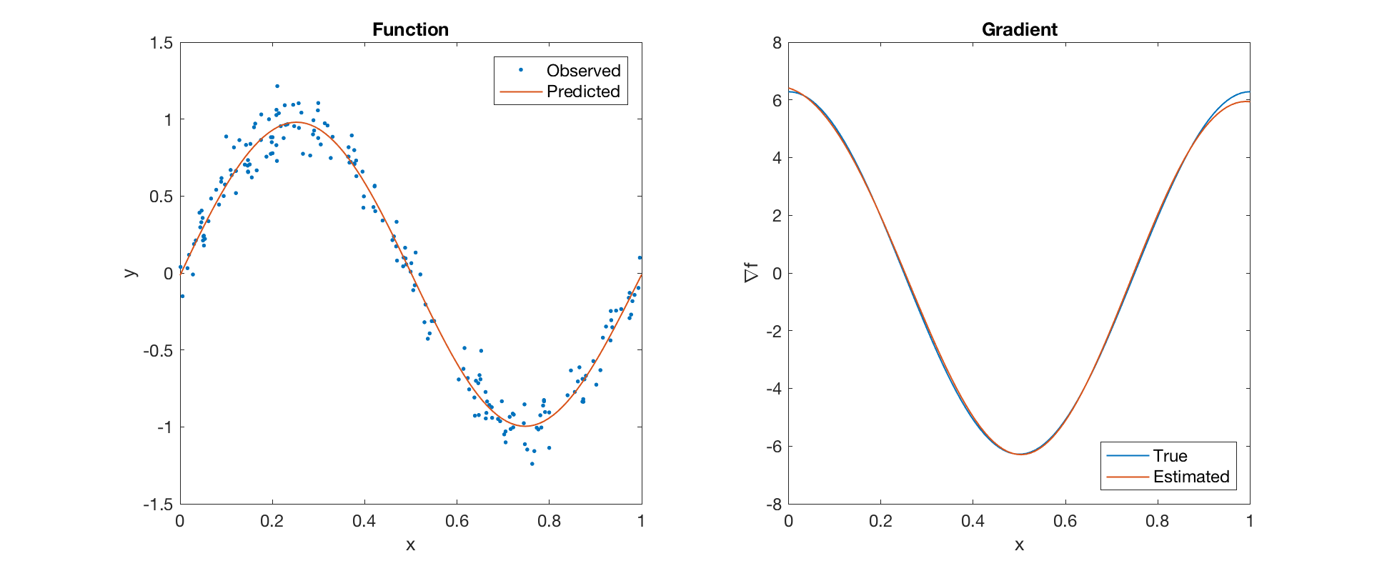
Here's an example for the 1d function $f(x) = \sin(2 \pi x)$. I fit a GPR model with squared exponential covariance function to 200 noisy observations. The noise variance and kernel parameters (signal variance and length-scale) were estimated by maximizing the marginal likelihood. The expected gradient (computed as above) is similar to the true gradient $\nabla f(x) = 2 \pi \cos (2 \pi x)$.

enter image description here

Gaussian process regression (GPR) gives a posterior distribution over functions mapping input to output. We can differentiate to obtain a distribution over the gradient. Below, I'll derive an expression for the expected gradient. There's no need to use finite differencing, as it can be computed in closed form (as long as the covariance function is differentiable; otherwise it doesn't exist).

Expression for the expected gradient

Assume the model:

$$y = f(\mathbf{x}) + \epsilon, \quad \epsilon \underset{\text{i.i.d.}}{\sim} \mathcal{N}(0, \sigma_n^2)$$

where the observed output $y \in \mathbb{R}$ is a function of input $\mathbf{x} \in \mathbb{R}^d$, plus i.i.d. Gaussian noise with variance $\sigma_n^2$. Say we fit a GPR model with differentiable covariance function $k$. Let $X = \{\mathbf{x_1}, \dots, \mathbf{x_n}\}$ denote the training inputs, and let $\mathbf{y} = [y_1, \dots, y_n]^T$ denote the corresponding training outputs. Let $\mathbf{x_*}$ denote a new input, and let $f_*$ be a random variable representing the function value at $\mathbf{x_*}$.

We want to compute $E[\nabla f_* \mid X, \mathbf{y}, \mathbf{x^*}]$, the expected gradient of the function evaluated at $\mathbf{x_*}$ (where the gradient is taken w.r.t. the input and the expectation is over the GPR posterior distribution). Because differentiation is a linear operation, this is equivalent to $\nabla E[ f_* \mid X, \mathbf{y}, \mathbf{x_*}]$, the gradient of the expected function value (i.e. posterior mean) at $\mathbf{x_*}$.

The expected function value at $\mathbf{x_*}$ is:

$$E[f_* \mid X, \mathbf{y}, \mathbf{x_*}] = \sum_{i=1}^n \alpha_i k(\mathbf{x_i}, \mathbf{x_*})$$

where $\mathbf{\alpha} = (K + \sigma_n^2 I)^{-1} \mathbf{y}$, $I$ is the identity matrix, and matrix $K$ contains the covariance for all pairs of training points ($K_{ij} = k(\mathbf{x_i}, \mathbf{x_j})$). For details, see chapter 2 of Rasmussen and Williams (2006).

Taking the gradient, we have:

$$\nabla E[f_* \mid X, \mathbf{y}, \mathbf{x_*}] = \nabla \sum_{i=1}^n \alpha_i \nabla k(\mathbf{x_*}, \mathbf{x_i})$$

$$= \sum_{i=1}^n \alpha_i \nabla k(\mathbf{x_*}, \mathbf{x_i})$$

Note that the weights $\mathbf{\alpha}$ are the same as used to compute the expected function value at $\mathbf{x^*}$. So, to compute the expected gradient, the only extra thing we need is the gradient of the covariance function.

For the squared exponential covariance function

As an example, the squared exponential (a.k.a. RBF) covariance function with signal variance $\sigma_f^2$ and length-scale $\ell$ is:

$$k(\mathbf{x}, \mathbf{x'}) = \sigma_f^2 \exp \left[ -\frac{\|\mathbf{x}-\mathbf{x'}\|^2}{2\ell^2} \right]$$

Taking $k(\mathbf{x_*}, \mathbf{x_i})$ and differentiating w.r.t. $\mathbf{x_*}$ gives:

$$\nabla k(\mathbf{x_*}, \mathbf{x_i}) = k(\mathbf{x_*}, \mathbf{x_i}) \frac{\mathbf{x_i} - \mathbf{x_*}}{\ell^2}$$

This can be plugged into the expression above for the expected gradient.

Example

Here's an example for the 1d function $f(x) = \sin(2 \pi x)$. I fit a GPR model with squared exponential covariance function to 200 noisy observations. The noise variance and kernel parameters (signal variance and length-scale) were estimated by maximizing the marginal likelihood. The expected gradient (computed as above) is similar to the true gradient $\nabla f(x) = 2 \pi \cos (2 \pi x)$.

enter image description here

Gaussian process regression (GPR) gives a posterior distribution over functions mapping input to output. We can differentiate to obtain a distribution over the gradient. Below, I'll derive an expression for the expected gradient. There's no need to use finite differencing, as it can be computed in closed form (as long as the covariance function is differentiable; otherwise it doesn't exist).

Expression for the expected gradient

Assume the model:

$$y = f(\mathbf{x}) + \epsilon, \quad \epsilon \underset{\text{i.i.d.}}{\sim} \mathcal{N}(0, \sigma_n^2)$$

where the observed output $y \in \mathbb{R}$ is a function of input $\mathbf{x} \in \mathbb{R}^d$, plus i.i.d. Gaussian noise with variance $\sigma_n^2$. Say we fit a GPR model with differentiable covariance function $k$. Let $X = \{\mathbf{x_1}, \dots, \mathbf{x_n}\}$ denote the training inputs, and let $\mathbf{y} = [y_1, \dots, y_n]^T$ denote the corresponding training outputs. Let $\mathbf{x_*}$ denote a new input, and let $f_*$ be a random variable representing the function value at $\mathbf{x_*}$.

We want to compute $E[\nabla f_* \mid X, \mathbf{y}, \mathbf{x^*}]$, the expected gradient of the function evaluated at $\mathbf{x_*}$ (where the gradient is taken w.r.t. the input and the expectation is over the GPR posterior distribution). Because differentiation is a linear operation, this is equivalent to $\nabla E[ f_* \mid X, \mathbf{y}, \mathbf{x_*}]$, the gradient of the expected function value (i.e. posterior mean) at $\mathbf{x_*}$.

The expected function value at $\mathbf{x_*}$ is:

$$E[f_* \mid X, \mathbf{y}, \mathbf{x_*}] = \sum_{i=1}^n \alpha_i k(\mathbf{x_i}, \mathbf{x_*})$$

where $\mathbf{\alpha} = (K + \sigma_n^2 I)^{-1} \mathbf{y}$, $I$ is the identity matrix, and matrix $K$ contains the covariance for all pairs of training points ($K_{ij} = k(\mathbf{x_i}, \mathbf{x_j})$). For details, see chapter 2 of Rasmussen and Williams (2006).

Taking the gradient, we have:

$$\nabla E[f_* \mid X, \mathbf{y}, \mathbf{x_*}] = \nabla \sum_{i=1}^n \alpha_i k(\mathbf{x_*}, \mathbf{x_i})$$

$$= \sum_{i=1}^n \alpha_i \nabla k(\mathbf{x_*}, \mathbf{x_i})$$

Note that the weights $\mathbf{\alpha}$ are the same as used to compute the expected function value at $\mathbf{x^*}$. So, to compute the expected gradient, the only extra thing we need is the gradient of the covariance function.

For the squared exponential covariance function

As an example, the squared exponential (a.k.a. RBF) covariance function with signal variance $\sigma_f^2$ and length-scale $\ell$ is:

$$k(\mathbf{x}, \mathbf{x'}) = \sigma_f^2 \exp \left[ -\frac{\|\mathbf{x}-\mathbf{x'}\|^2}{2\ell^2} \right]$$

Taking $k(\mathbf{x_*}, \mathbf{x_i})$ and differentiating w.r.t. $\mathbf{x_*}$ gives:

$$\nabla k(\mathbf{x_*}, \mathbf{x_i}) = k(\mathbf{x_*}, \mathbf{x_i}) \frac{\mathbf{x_i} - \mathbf{x_*}}{\ell^2}$$

This can be plugged into the expression above for the expected gradient.

Example

Here's an example for the 1d function $f(x) = \sin(2 \pi x)$. I fit a GPR model with squared exponential covariance function to 200 noisy observations. The noise variance and kernel parameters (signal variance and length-scale) were estimated by maximizing the marginal likelihood. The expected gradient (computed as above) is similar to the true gradient $\nabla f(x) = 2 \pi \cos (2 \pi x)$.

enter image description here

Source Link
user20160
  • 33.2k
  • 3
  • 82
  • 114

Gaussian process regression (GPR) gives a posterior distribution over functions mapping input to output. We can differentiate to obtain a distribution over the gradient. Below, I'll derive an expression for the expected gradient. There's no need to use finite differencing, as it can be computed in closed form (as long as the covariance function is differentiable; otherwise it doesn't exist).

Expression for the expected gradient

Assume the model:

$$y = f(\mathbf{x}) + \epsilon, \quad \epsilon \underset{\text{i.i.d.}}{\sim} \mathcal{N}(0, \sigma_n^2)$$

where the observed output $y \in \mathbb{R}$ is a function of input $\mathbf{x} \in \mathbb{R}^d$, plus i.i.d. Gaussian noise with variance $\sigma_n^2$. Say we fit a GPR model with differentiable covariance function $k$. Let $X = \{\mathbf{x_1}, \dots, \mathbf{x_n}\}$ denote the training inputs, and let $\mathbf{y} = [y_1, \dots, y_n]^T$ denote the corresponding training outputs. Let $\mathbf{x_*}$ denote a new input, and let $f_*$ be a random variable representing the function value at $\mathbf{x_*}$.

We want to compute $E[\nabla f_* \mid X, \mathbf{y}, \mathbf{x^*}]$, the expected gradient of the function evaluated at $\mathbf{x_*}$ (where the gradient is taken w.r.t. the input and the expectation is over the GPR posterior distribution). Because differentiation is a linear operation, this is equivalent to $\nabla E[ f_* \mid X, \mathbf{y}, \mathbf{x_*}]$, the gradient of the expected function value (i.e. posterior mean) at $\mathbf{x_*}$.

The expected function value at $\mathbf{x_*}$ is:

$$E[f_* \mid X, \mathbf{y}, \mathbf{x_*}] = \sum_{i=1}^n \alpha_i k(\mathbf{x_i}, \mathbf{x_*})$$

where $\mathbf{\alpha} = (K + \sigma_n^2 I)^{-1} \mathbf{y}$, $I$ is the identity matrix, and matrix $K$ contains the covariance for all pairs of training points ($K_{ij} = k(\mathbf{x_i}, \mathbf{x_j})$). For details, see chapter 2 of Rasmussen and Williams (2006).

Taking the gradient, we have:

$$\nabla E[f_* \mid X, \mathbf{y}, \mathbf{x_*}] = \nabla \sum_{i=1}^n \alpha_i \nabla k(\mathbf{x_*}, \mathbf{x_i})$$

$$= \sum_{i=1}^n \alpha_i \nabla k(\mathbf{x_*}, \mathbf{x_i})$$

Note that the weights $\mathbf{\alpha}$ are the same as used to compute the expected function value at $\mathbf{x^*}$. So, to compute the expected gradient, the only extra thing we need is the gradient of the covariance function.

For the squared exponential covariance function

As an example, the squared exponential (a.k.a. RBF) covariance function with signal variance $\sigma_f^2$ and length-scale $\ell$ is:

$$k(\mathbf{x}, \mathbf{x'}) = \sigma_f^2 \exp \left[ -\frac{\|\mathbf{x}-\mathbf{x'}\|^2}{2\ell^2} \right]$$

Taking $k(\mathbf{x_*}, \mathbf{x_i})$ and differentiating w.r.t. $\mathbf{x_*}$ gives:

$$\nabla k(\mathbf{x_*}, \mathbf{x_i}) = k(\mathbf{x_*}, \mathbf{x_i}) \frac{\mathbf{x_i} - \mathbf{x_*}}{\ell^2}$$

This can be plugged into the expression above for the expected gradient.

Example

Here's an example for the 1d function $f(x) = \sin(2 \pi x)$. I fit a GPR model with squared exponential covariance function to 200 noisy observations. The noise variance and kernel parameters (signal variance and length-scale) were estimated by maximizing the marginal likelihood. The expected gradient (computed as above) is similar to the true gradient $\nabla f(x) = 2 \pi \cos (2 \pi x)$.

enter image description here