more explanation
Source Link
GiorgioG
  • 111
  • 1
  • 7
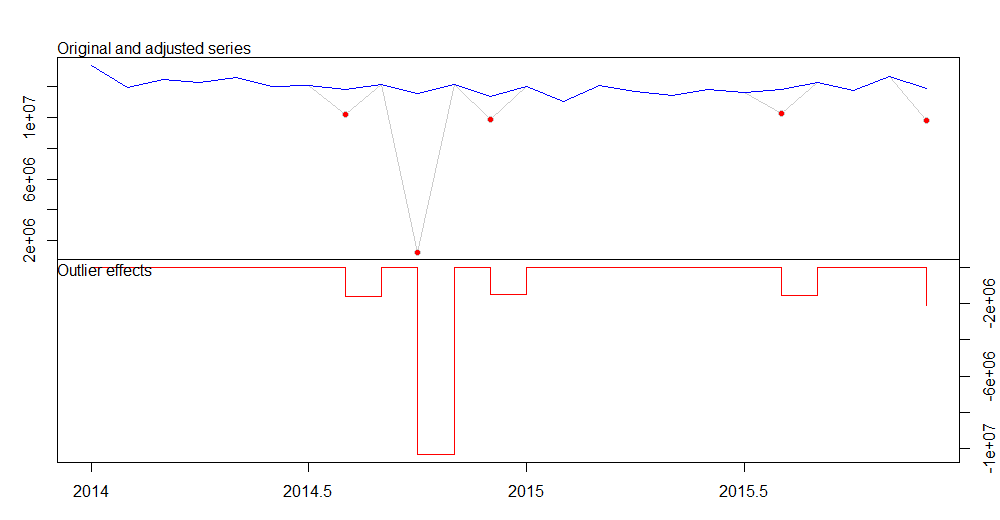
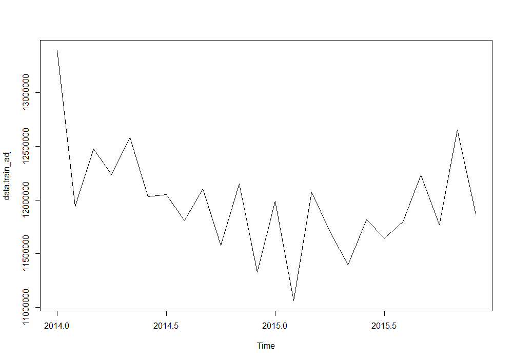
This is the outliers adjusted time series.

data.train_adj <- tso_res$yadj
plot(data.train_adj)

We can see both data.train and data.train_adj.

> data.train
          Jan      Feb      Mar      Apr      May      Jun      Jul      Aug      Sep      Oct      Nov      Dec
2014 13392905 11939873 12473667 12237110 12579693 12030095 12052101 10205025 12102526  1237336 12148331  9842860
2015 11990085 11061740 12076397 11702514 11395657 11817594 11643682 10243241 12233001 11769231 12652418  9774333
> data.train_adj
          Jan      Feb      Mar      Apr      May      Jun      Jul      Aug      Sep      Oct      Nov      Dec
2014 13392905 11939873 12473667 12237110 12579693 12030095 12052101 11807296 12102526 11576627 12148331 11329957
2015 11990085 11061740 12076397 11702514 11395657 11817594 11643682 11795494 12233001 11769231 12652418 11869616

To accomplish with your need to capture seasonality, I take advantage of dynamic harmonic regression within ARIMA modeling. You may determine an optimal number of Fourier sin and cos pairs number (K) by trying out a pool of values for and select the one with minimum AICc. Here I show it with K=4. Please note that Fourier coefficients are actually not statistically significative as their standard deviations compaired to the coefficients value show.

data.train_adj <- tso_res$yadj
plot(data.train_adj)

To accomplish with your need to capture seasonality, I take advantage of dynamic harmonic regression within ARIMA modeling. You may determine an optimal number of Fourier sin and cos pairs number (K) by trying out a pool of values for and select the one with minimum AICc. Here I show it with K=4.

This is the outliers adjusted time series.

data.train_adj <- tso_res$yadj
plot(data.train_adj)

We can see both data.train and data.train_adj.

> data.train
          Jan      Feb      Mar      Apr      May      Jun      Jul      Aug      Sep      Oct      Nov      Dec
2014 13392905 11939873 12473667 12237110 12579693 12030095 12052101 10205025 12102526  1237336 12148331  9842860
2015 11990085 11061740 12076397 11702514 11395657 11817594 11643682 10243241 12233001 11769231 12652418  9774333
> data.train_adj
          Jan      Feb      Mar      Apr      May      Jun      Jul      Aug      Sep      Oct      Nov      Dec
2014 13392905 11939873 12473667 12237110 12579693 12030095 12052101 11807296 12102526 11576627 12148331 11329957
2015 11990085 11061740 12076397 11702514 11395657 11817594 11643682 11795494 12233001 11769231 12652418 11869616

To accomplish with your need to capture seasonality, I take advantage of dynamic harmonic regression within ARIMA modeling. You may determine an optimal number of Fourier sin and cos pairs number (K) by trying out a pool of values for and select the one with minimum AICc. Here I show it with K=4. Please note that Fourier coefficients are actually not statistically significative as their standard deviations compaired to the coefficients value show.
Source Link
GiorgioG
  • 111
  • 1
  • 7

library(forecast)
library(tsoutliers)

data.train<-window(mydata_ts,start=c(2014,1),end=c(2015,12))
data.test<-window(mydata_ts,start=c(2016,1))

tso_res <- tso(data.train)
tso_res

Series: data.train 
Regression with ARIMA(1,1,0) errors 

Coefficients:
          ar1         AO8         AO10      AO12        AO20        AO24
      -0.8863  -1602271.0  -10339290.5  -1487097  -1552253.1  -2095283.0
s.e.   0.1156    332809.5     384994.5    334836    272327.7    379263.1

sigma^2 estimated as 1.805e+11:  log likelihood=-327.99
AIC=669.99   AICc=677.45   BIC=677.94

Outliers:
  type ind    time   coefhat   tstat
1   AO   8 2014:08  -1602271  -4.814
2   AO  10 2014:10 -10339291 -26.856
3   AO  12 2014:12  -1487097  -4.441
4   AO  20 2015:08  -1552253  -5.700
5   AO  24 2015:12  -2095283  -5.525

plot(tso_res)

enter image description here

data.train_adj <- tso_res$yadj
plot(data.train_adj)

enter image description here

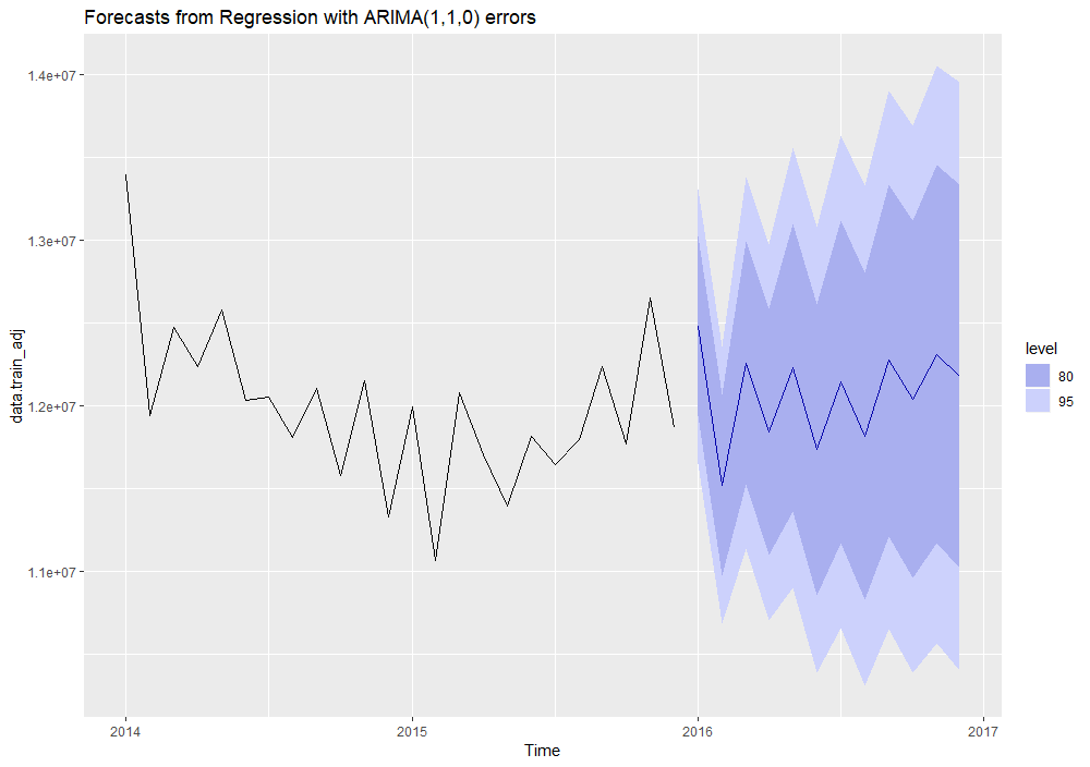
To accomplish with your need to capture seasonality, I take advantage of dynamic harmonic regression within ARIMA modeling. You may determine an optimal number of Fourier sin and cos pairs number (K) by trying out a pool of values for and select the one with minimum AICc. Here I show it with K=4.

model_auto <- auto.arima(data.train_adj, trace=TRUE,  ic="aic", stepwise = FALSE, xreg= fourier(data.train_adj, K = 4))
model_auto

Series: data.train_adj 
Regression with ARIMA(1,1,0) errors 

Coefficients:
          ar1      S1-12     C1-12      S2-12     C2-12     S3-12     C3-12    S4-12     C4-12
      -0.8934  -59902.58  101672.4  -81457.95  35595.59  20279.40  67730.84  47447.4  22978.35
s.e.   0.1028  112888.52  102427.8   63037.36  60833.99  53262.02  53310.64  61555.9  60441.30

sigma^2 estimated as 1.799e+11:  log likelihood=-325.75
AIC=671.51   AICc=689.84   BIC=682.86


autoplot(forecast(model_auto, xreg=fourier(data.train_adj, K=4, h=12)))

enter image description here