addition after the question has bit editet
Source Link
Pere
  • 6.6k
  • 1
  • 18
  • 34

Experienced practitioners know the usual aspect of every graph and are able to tell whether (and how) a given graph deviates from the usual case. Since I'm not an experienced practitioner, I need to generate benchmark graphics to compare with my problem graphics. This way it's easier to tell if the situation depicted in a given graph is different from the expected situation I have simulated.

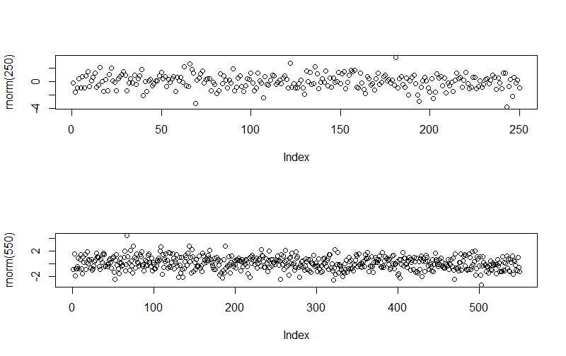
Faced with your problem, I would try to simulate a graph of residuals from an homoskedastic population and compare it with your graphs. The problem now is that we need to know what distribution are we going to sample from. Any insight on what distribution residuals are expected to follow in your problem would be very useful. However, since I don't have such insight, I would start trying with a normal distribution:

par(mfrow=c(2,1))
plot(rnorm(250))
plot(rnorm(550))

gausian residuals

Just by comparing with those graphs I would say:

  • Some outliers can be expected even in an homoskedastic distribution.
  • Your outliers are a lot more far away than mine. If your residuals are supposed to be normally distributed, that could be a symptom of heteroskedacity. However, it could also be just a symptom that residuals follow a distribution with heavy tails.

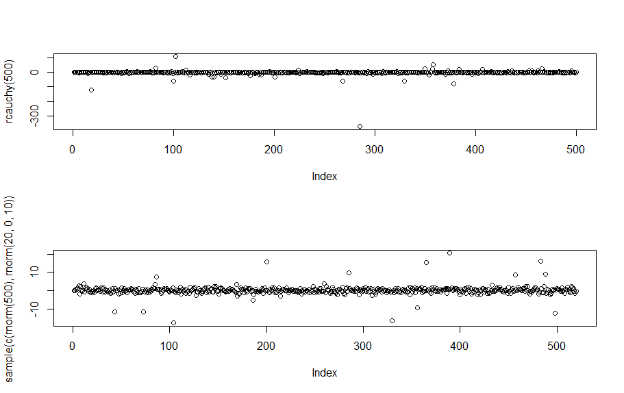
Let's try what happens with a couple of heavy-tailed distributions:

plot(rcauchy(500))
plot(sample(c(rnorm(500),rnorm(20,0,10))))

heavy tailed residuals

Those look a lot more similar to your graphs - in fact, there are a few places where we could add green ellipses like yours.

Therefore, although formal tests allow to diagnose more accurately (as Michael Grogan points in his answer), I would say that your residuals don't look like coming from a Gaussian distribution with uniform variance. If they are supposed to be Gaussian, they may be heteroskedastic (or have another problem). If they aren't supposed to be Gaussian, they may just be following a heavy-tailed distribution with uniform variance.

Addition after edit in question:

In the UCG series I see a many periods of several days or weeks with no visible change with days of dramatic changes between days. This leads to a dUCG series with a lot of zero (or maybe near zero) values. With such data most models are likely to get good fits in the quiet periods and large residuals for the fast moving days. Therefore, residuals are likely to follow a heavy tailed distribution and I wouldn't attribute to heteroskedacity the outliers you marked with green ellipses.

Experienced practitioners know the usual aspect of every graph and are able to tell whether (and how) a given graph deviates from the usual case. Since I'm not an experienced practitioner, I need to generate benchmark graphics to compare with my problem graphics. This way it's easier to tell if the situation depicted in a given graph is different from the expected situation I have simulated.

Faced with your problem, I would try to simulate a graph of residuals from an homoskedastic population and compare it with your graphs. The problem now is that we need to know what distribution are we going to sample from. Any insight on what distribution residuals are expected to follow in your problem would be very useful. However, since I don't have such insight, I would start trying with a normal distribution:

par(mfrow=c(2,1))
plot(rnorm(250))
plot(rnorm(550))

gausian residuals

Just by comparing with those graphs I would say:

  • Some outliers can be expected even in an homoskedastic distribution.
  • Your outliers are a lot more far away than mine. If your residuals are supposed to be normally distributed, that could be a symptom of heteroskedacity. However, it could also be just a symptom that residuals follow a distribution with heavy tails.

Let's try what happens with a couple of heavy-tailed distributions:

plot(rcauchy(500))
plot(sample(c(rnorm(500),rnorm(20,0,10))))

heavy tailed residuals

Those look a lot more similar to your graphs - in fact, there are a few places where we could add green ellipses like yours.

Therefore, although formal tests allow to diagnose more accurately (as Michael Grogan points in his answer), I would say that your residuals don't look like coming from a Gaussian distribution with uniform variance. If they are supposed to be Gaussian, they may be heteroskedastic (or have another problem). If they aren't supposed to be Gaussian, they may just be following a heavy-tailed distribution with uniform variance.

Addition after edit in question:

In the UCG series I see a many periods of several days or weeks with no visible change with days of dramatic changes between days. This leads to a dUCG series with a lot of zero (or maybe near zero) values. With such data most models are likely to get good fits in the quiet periods and large residuals for the fast moving days. Therefore, residuals are likely to follow a heavy tailed distribution and I wouldn't attribute to heteroskedacity the outliers you marked with green ellipses.
Source Link
Pere
  • 6.6k
  • 1
  • 18
  • 34

Experienced practitioners know the usual aspect of every graph and are able to tell whether (and how) a given graph deviates from the usual case. Since I'm not an experienced practitioner, I need to generate benchmark graphics to compare with my problem graphics. This way it's easier to tell if the situation depicted in a given graph is different from the expected situation I have simulated.

Faced with your problem, I would try to simulate a graph of residuals from an homoskedastic population and compare it with your graphs. The problem now is that we need to know what distribution are we going to sample from. Any insight on what distribution residuals are expected to follow in your problem would be very useful. However, since I don't have such insight, I would start trying with a normal distribution:

par(mfrow=c(2,1))
plot(rnorm(250))
plot(rnorm(550))

gausian residuals

Just by comparing with those graphs I would say:

  • Some outliers can be expected even in an homoskedastic distribution.
  • Your outliers are a lot more far away than mine. If your residuals are supposed to be normally distributed, that could be a symptom of heteroskedacity. However, it could also be just a symptom that residuals follow a distribution with heavy tails.

Let's try what happens with a couple of heavy-tailed distributions:

plot(rcauchy(500))
plot(sample(c(rnorm(500),rnorm(20,0,10))))

heavy tailed residuals

Those look a lot more similar to your graphs - in fact, there are a few places where we could add green ellipses like yours.

Therefore, although formal tests allow to diagnose more accurately (as Michael Grogan points in his answer), I would say that your residuals don't look like coming from a Gaussian distribution with uniform variance. If they are supposed to be Gaussian, they may be heteroskedastic (or have another problem). If they aren't supposed to be Gaussian, they may just be following a heavy-tailed distribution with uniform variance.