My answer will focus on the baseline OLS case, but the mechanics are similar for techniques like Lasso (although I'll admit that I do not know how $R^2$ is computed for such methods). Also, my answer relates to in-sample fit.
Recall that $R^2$ is defined as (also recall that the mean of the fitted values equals the mean of the $y$, $\bar y=\bar{\hat{y}}$) $$ R^2=\frac{(\hat y-\bar y)'(\hat y-\bar y)}{(y-\bar y)'(y-\bar y)}, $$ which we may rewrite into the ratio of variance explained to variance of the dependent variable, $$ R^2=\frac{\frac{1}{n-1}\sum_i(\hat y_i-\bar y)^2}{\frac{1}{n-1}\sum_i( y_i-\bar y)^2}, $$$$ R^2=\frac{\frac{1}{n-1}\sum_i(\hat y_i-\bar y)^2}{\frac{1}{n-1}\sum_i( y_i-\bar y)^2}=\frac{\hat\sigma^2_{\hat y}}{\hat\sigma^2_{y}}, $$ So, when you have a low $R^2$, that is tantamount to saying that the standard deviation of the predictions is less than the standard deviation of the target variable. A fortiori, if you "sacrifice" $R^2$, that ratio can only decrease further.
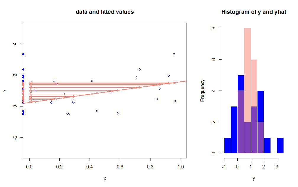
Here is a little graphical illustration, in which both the $y_i$ (blue) and the fitted values (salmon) are projected onto the y-axis, for a dataset in which $R^2$ is relatively low. We observe that the variation of the fitted values is, as expected, smaller.

