What seems to work, and what I ended up doing, was to define a new sampling distribution using the "ones trick" described in the BUGS manual and with and example for jags given here.

For the "ones" trick to work I need to define the likelihood function for my new distribution, which is the same as the [probability density function] but with the data as the variable argument instead of the parameters.

Using the following equality, where $X$ and $Y$ are random variables and $x$ is a constant:

$ prob(min(X, Y)>x) = prob(X>x\ and\ Y>x) = prob(X>x) \cdot prob(Y>x) $

I can construct the cumulative density function for my special distribution as follows:

$ prob(min(norm1, norm2) < x) \Rightarrow 1 - prob(min(norm1, norm2) > x) \Rightarrow 1 - prob(norm1 > x\ and\ norm2 > x) \Rightarrow 1 - prob(norm1>x) \cdot prob(norm2>x) \Rightarrow 1 - (1 - prob(norm1<x)) \cdot (1 - prob(norm2<x))$

As $prob(norm1 < z)$ is the cumulative density function of a normal distribution the final "special" cumulative density function is:

$1 - (1 - pnorm(x,\mu_1, \sigma_1)) \cdot (1-pnorm(x,\mu_2, \sigma_2))$

To get the probability density function I deviatedifferentiate this using the equalityproduct rule:

$ h(x)=f_1(x)*f_2(x) \Rightarrow h'(x) = f_2'(x)*f_1(x) + f_1'(x)*f_2(x)$

and end up with the following R expression:

-(-dnorm(x, m1, s1) * (1 - pnorm(x, m2, s2)) + -dnorm(x, m2, s2) * (1 - pnorm(x, m1, s1)))

In jags the final model specification became (notice that s1 has become 1/pow(s1, 2) due to jags using precision instead of SD):

model{
    for (i in 1:n){
    p[i] <- -(-dnorm(x[i], m1, 1/pow(s1, 2)) * (1 - pnorm(x[i], m2, 1/pow(s2, 2))) + -dnorm(x[i], m2, 1/pow(s2, 2)) * (1 - pnorm(x[i], m1, 1/pow(s1, 2))))
    ones[i] ~ dbern(p[i])
    }
    m1_sd <- 1000
    m1 ~ dnorm(0, 1/pow(m1_sd, 2))
    m2_sd <- 1000
    m2 ~ dnorm(400, 1/pow(m2_sd, 2))
    s1_m <- 400 
    s1_s <- 1000
    s1 ~ dgamma(pow(s1_m,2)/pow(s1_s,2), s1_m/pow(s1_s,2))
    s2_m <- 100 
    s2_s <- 1000
    s2 ~ dgamma(pow(s2_m,2)/pow(s2_s,2), s2_m/pow(s2_s,2))
}

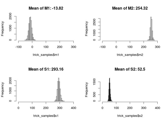
This model seems to (and should) retrieve the original parameters as the following 10000 sample posteriors show: posterior plot
What seems to work, and what I ended up doing, was to define a new sampling distribution using the "ones trick" described in the BUGS manual and with and example for jags given here.

For the "ones" trick to work I need to define the likelihood function for my new distribution, which is the same as the [probability density function] but with the data as the variable argument instead of the parameters.

Using the following equality, where $X$ and $Y$ are random variables and $x$ is a constant:

$ prob(min(X, Y)>x) = prob(X>x\ and\ Y>x) = prob(X>x) \cdot prob(Y>x) $

I can construct the cumulative density function for my special distribution as follows:

$ prob(min(norm1, norm2) < x) \Rightarrow 1 - prob(min(norm1, norm2) > x) \Rightarrow 1 - prob(norm1 > x\ and\ norm2 > x) \Rightarrow 1 - prob(norm1>x) \cdot prob(norm2>x) \Rightarrow 1 - (1 - prob(norm1<x)) \cdot (1 - prob(norm2<x))$

As $prob(norm1 < z)$ is the cumulative density function of a normal distribution the final "special" cumulative density function is:

$1 - (1 - pnorm(x,\mu_1, \sigma_1)) \cdot (1-pnorm(x,\mu_2, \sigma_2))$

To get the probability density function I deviate this using the equality:

$ h(x)=f_1(x)*f_2(x) \Rightarrow h'(x) = f_2'(x)*f_1(x) + f_1'(x)*f_2(x)$

and end up with the following R expression:

-(-dnorm(x, m1, s1) * (1 - pnorm(x, m2, s2)) + -dnorm(x, m2, s2) * (1 - pnorm(x, m1, s1)))

In jags the final model specification became (notice that s1 has become 1/pow(s1, 2) due to jags using precision instead of SD):

model{
    for (i in 1:n){
    p[i] <- -(-dnorm(x[i], m1, 1/pow(s1, 2)) * (1 - pnorm(x[i], m2, 1/pow(s2, 2))) + -dnorm(x[i], m2, 1/pow(s2, 2)) * (1 - pnorm(x[i], m1, 1/pow(s1, 2))))
    ones[i] ~ dbern(p[i])
    }
    m1_sd <- 1000
    m1 ~ dnorm(0, 1/pow(m1_sd, 2))
    m2_sd <- 1000
    m2 ~ dnorm(400, 1/pow(m2_sd, 2))
    s1_m <- 400 
    s1_s <- 1000
    s1 ~ dgamma(pow(s1_m,2)/pow(s1_s,2), s1_m/pow(s1_s,2))
    s2_m <- 100 
    s2_s <- 1000
    s2 ~ dgamma(pow(s2_m,2)/pow(s2_s,2), s2_m/pow(s2_s,2))
}

This model seems to (and should) retrieve the original parameters as the following 10000 sample posteriors show: posterior plot

What seems to work, and what I ended up doing, was to define a new sampling distribution using the "ones trick" described in the BUGS manual and with and example for jags given here.

For the "ones" trick to work I need to define the likelihood function for my new distribution, which is the same as the [probability density function] but with the data as the variable argument instead of the parameters.

Using the following equality, where $X$ and $Y$ are random variables and $x$ is a constant:

$ prob(min(X, Y)>x) = prob(X>x\ and\ Y>x) = prob(X>x) \cdot prob(Y>x) $

I can construct the cumulative density function for my special distribution as follows:

$ prob(min(norm1, norm2) < x) \Rightarrow 1 - prob(min(norm1, norm2) > x) \Rightarrow 1 - prob(norm1 > x\ and\ norm2 > x) \Rightarrow 1 - prob(norm1>x) \cdot prob(norm2>x) \Rightarrow 1 - (1 - prob(norm1<x)) \cdot (1 - prob(norm2<x))$

As $prob(norm1 < z)$ is the cumulative density function of a normal distribution the final "special" cumulative density function is:

$1 - (1 - pnorm(x,\mu_1, \sigma_1)) \cdot (1-pnorm(x,\mu_2, \sigma_2))$

To get the probability density function I differentiate this using the product rule:

$ h(x)=f_1(x)*f_2(x) \Rightarrow h'(x) = f_2'(x)*f_1(x) + f_1'(x)*f_2(x)$

and end up with the following R expression:

-(-dnorm(x, m1, s1) * (1 - pnorm(x, m2, s2)) + -dnorm(x, m2, s2) * (1 - pnorm(x, m1, s1)))

In jags the final model specification became (notice that s1 has become 1/pow(s1, 2) due to jags using precision instead of SD):

model{
    for (i in 1:n){
    p[i] <- -(-dnorm(x[i], m1, 1/pow(s1, 2)) * (1 - pnorm(x[i], m2, 1/pow(s2, 2))) + -dnorm(x[i], m2, 1/pow(s2, 2)) * (1 - pnorm(x[i], m1, 1/pow(s1, 2))))
    ones[i] ~ dbern(p[i])
    }
    m1_sd <- 1000
    m1 ~ dnorm(0, 1/pow(m1_sd, 2))
    m2_sd <- 1000
    m2 ~ dnorm(400, 1/pow(m2_sd, 2))
    s1_m <- 400 
    s1_s <- 1000
    s1 ~ dgamma(pow(s1_m,2)/pow(s1_s,2), s1_m/pow(s1_s,2))
    s2_m <- 100 
    s2_s <- 1000
    s2 ~ dgamma(pow(s2_m,2)/pow(s2_s,2), s2_m/pow(s2_s,2))
}

This model seems to (and should) retrieve the original parameters as the following 10000 sample posteriors show: posterior plot

Source Link
Rasmus Bååth
  • 6.9k
  • 41
  • 58

What seems to work, and what I ended up doing, was to define a new sampling distribution using the "ones trick" described in the BUGS manual and with and example for jags given here.

For the "ones" trick to work I need to define the likelihood function for my new distribution, which is the same as the [probability density function] but with the data as the variable argument instead of the parameters.

Using the following equality, where $X$ and $Y$ are random variables and $x$ is a constant:

$ prob(min(X, Y)>x) = prob(X>x\ and\ Y>x) = prob(X>x) \cdot prob(Y>x) $

I can construct the cumulative density function for my special distribution as follows:

$ prob(min(norm1, norm2) < x) \Rightarrow 1 - prob(min(norm1, norm2) > x) \Rightarrow 1 - prob(norm1 > x\ and\ norm2 > x) \Rightarrow 1 - prob(norm1>x) \cdot prob(norm2>x) \Rightarrow 1 - (1 - prob(norm1<x)) \cdot (1 - prob(norm2<x))$

As $prob(norm1 < z)$ is the cumulative density function of a normal distribution the final "special" cumulative density function is:

$1 - (1 - pnorm(x,\mu_1, \sigma_1)) \cdot (1-pnorm(x,\mu_2, \sigma_2))$

To get the probability density function I deviate this using the equality:

$ h(x)=f_1(x)*f_2(x) \Rightarrow h'(x) = f_2'(x)*f_1(x) + f_1'(x)*f_2(x)$

and end up with the following R expression:

-(-dnorm(x, m1, s1) * (1 - pnorm(x, m2, s2)) + -dnorm(x, m2, s2) * (1 - pnorm(x, m1, s1)))

In jags the final model specification became (notice that s1 has become 1/pow(s1, 2) due to jags using precision instead of SD):

model{
    for (i in 1:n){
    p[i] <- -(-dnorm(x[i], m1, 1/pow(s1, 2)) * (1 - pnorm(x[i], m2, 1/pow(s2, 2))) + -dnorm(x[i], m2, 1/pow(s2, 2)) * (1 - pnorm(x[i], m1, 1/pow(s1, 2))))
    ones[i] ~ dbern(p[i])
    }
    m1_sd <- 1000
    m1 ~ dnorm(0, 1/pow(m1_sd, 2))
    m2_sd <- 1000
    m2 ~ dnorm(400, 1/pow(m2_sd, 2))
    s1_m <- 400 
    s1_s <- 1000
    s1 ~ dgamma(pow(s1_m,2)/pow(s1_s,2), s1_m/pow(s1_s,2))
    s2_m <- 100 
    s2_s <- 1000
    s2 ~ dgamma(pow(s2_m,2)/pow(s2_s,2), s2_m/pow(s2_s,2))
}

This model seems to (and should) retrieve the original parameters as the following 10000 sample posteriors show: posterior plot