I'd like to understand why my partial dependence plots for a logistic regression model simply show up as straight lines -- even when I'd expect basically a threshold effect from a covariate. I know partial dependence plots are typical of machine learning, but the (excellent) description by the authors of the pdp] package suggest glms are fair game. So why does the relationship between outcome and effort (below) appear to be linear?

Here's a dummy dataset. Note that I forced higher values of effort for outcomes corresponding to 1 (a "win"). Also note that sometimes the algorithm won't converge -- if that's the case, just generate new data.

# Sample game data
outcome <- as.vector(cbind(rep(0,25), rep(1,25)))
effort <- as.vector(cbind(rnorm(25, 25, 5), rnorm(25, 50, 10)))
skill <- rnorm(50, 50, 20)
game <- cbind(outcome, effort, skill) %>% as.data.frame()

# Simple glm
mod <- glm(outcome ~ effort + skill, data = game, family = binomial(link = "logit"))
summary(mod)
partial(mod, pred.var = c("effort"), plot = TRUE)

Call:
glm(formula = outcome ~ effort + skill, family = binomial(link = "logit"), 
    data = game)

Deviance Residuals: 
     Min        1Q    Median        3Q       Max  
-1.26979  -0.13985  -0.00751   0.01736   2.34734  

Coefficients:
             Estimate Std. Error z value Pr(>|z|)   
(Intercept) -15.12758    5.73393  -2.638  0.00833 **
effort        0.50174    0.19218   2.611  0.00903 **
skill        -0.05414    0.05142  -1.053  0.29231   

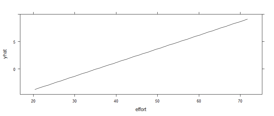
Clearly, effort is going to be a strong predictor -- with way more wins (1s) associated with higher effort (given my data assignments). However, the partial dependence plot looks like this:

partial(mod, pred.var = c("effort"), plot = TRUE)

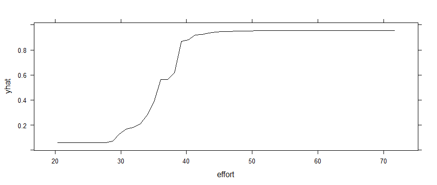
If I use a random forest instead, that threshold effect shows up. (Yes, I know it throws a warning about using <5 unique response values in regression. It also shows up if you force outcome to be a factor.)

rf <- randomForest(outcome ~ effort + skill, data = game)
partial(rf, pred.var = c("effort"), plot = TRUE)

My primary question here is not about which model is a better fit, but why the partial dependence is apparently linear with the logistic regression? Why doesn't that 30-40 range pop out as a threshold in the glm plot? Is that truly representing the relationship between game and effort in the model?

Thanks for any insights!