added 276 characters in body
Source Link
BruceET
  • 57.6k
  • 2
  • 36
  • 94

A quick answer based on the links (and corresponding references) in Comments: Use a Bayesian probability interval (based on a flatuniform prior) to serve as a frequentist confidence interval (CI).

If you have $X = 3$ successes in $n = 275$ trials, then your 95% CI can be found in R as qbeta(c(.025, .975), x + 1, n - x + 1):

x = 3;  n = 275
qbeta(c(.025,.975), x+1, n-x+1)
[1] 0.003962534 0.031435106

So you might use $(0.004,\,0.031)$ as your 95% CI.

Notes: (a) The Jeffrey's interval mentioned in references uses 1/10.5 where I have used 1. That is

 x = 3;  n = 275
 qbeta(c(.025,.975), x+.5, n-x+.5)
 [1] 0.003081784 0.028823996

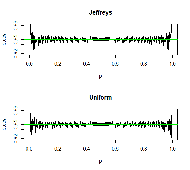
Most of the time, the two intervals are almost the same. In my experience, using the flatuniform prior instead of the Jeffreys prior happens to give betterslightly more consistent coverage probabilities in a few isolatedsome cases forof proportions very near 0 or 1. Plots of coverage probabilities for $n = 275$ are shown below:

enter image description here

(b) If you're using software other than R, qbeta is the an inverse CDF function (quantile function) for a beta random variable. Most commercial programs can be used to get the same result (even if not as compactly as R). For example, using Minitab we get:

MTB > invcdf .025;
SUBC> beta 4 273.

Inverse Cumulative Distribution Function 
Beta with first shape parameter = 4 and second = 273
P( X ≤ x )          x
     0.025  0.0039625

MTB > invcdf .975;
SUBC> beta 4 273.

Inverse Cumulative Distribution Function 
Beta with first shape parameter = 4 and second = 273
P( X ≤ x )          x
     0.975  0.0314351

A quick answer based on the links (and corresponding references) in Comments: Use a Bayesian probability interval (based on a flat prior) to serve as a frequentist confidence interval (CI).

If you have $X = 3$ successes in $n = 275$ trials, then your 95% CI can be found in R as qbeta(c(.025, .975), x + 1, n - x + 1):

x = 3;  n = 275
qbeta(c(.025,.975), x+1, n-x+1)
[1] 0.003962534 0.031435106

So you might use $(0.004,\,0.031)$ as your 95% CI.

Notes: (a) The Jeffrey's interval mentioned in references uses 1/1 where I have used 1. That is

 x = 3;  n = 275
 qbeta(c(.025,.975), x+.5, n-x+.5)
 [1] 0.003081784 0.028823996

Most of the time, the two intervals are almost the same. In my experience, using the flat prior instead of the Jeffreys prior happens to give better coverage in a few isolated cases for proportions near 0 or 1.

(b) If you're using software other than R, qbeta is the an inverse CDF function (quantile function) for a beta random variable. Most commercial programs can be used to get the same result (even if not as compactly as R). For example, using Minitab we get:

MTB > invcdf .025;
SUBC> beta 4 273.

Inverse Cumulative Distribution Function 
Beta with first shape parameter = 4 and second = 273
P( X ≤ x )          x
     0.025  0.0039625

MTB > invcdf .975;
SUBC> beta 4 273.

Inverse Cumulative Distribution Function 
Beta with first shape parameter = 4 and second = 273
P( X ≤ x )          x
     0.975  0.0314351
A quick answer based on the links (and corresponding references) in Comments: Use a Bayesian probability interval (based on a uniform prior) to serve as a frequentist confidence interval (CI).

If you have $X = 3$ successes in $n = 275$ trials, then your 95% CI can be found in R as qbeta(c(.025, .975), x + 1, n - x + 1):

x = 3;  n = 275
qbeta(c(.025,.975), x+1, n-x+1)
[1] 0.003962534 0.031435106

So you might use $(0.004,\,0.031)$ as your 95% CI.

Notes: (a) The Jeffrey's interval mentioned in references uses 0.5 where I have used 1. That is

 x = 3;  n = 275
 qbeta(c(.025,.975), x+.5, n-x+.5)
 [1] 0.003081784 0.028823996

Most of the time, the two intervals are almost the same. In my experience, using the uniform prior instead of the Jeffreys prior happens to give slightly more consistent coverage probabilities in some cases of proportions very near 0 or 1. Plots of coverage probabilities for $n = 275$ are shown below:

enter image description here

(b) If you're using software other than R, qbeta is the an inverse CDF function (quantile function) for a beta random variable. Most commercial programs can be used to get the same result (even if not as compactly as R). For example, using Minitab we get:

MTB > invcdf .025;
SUBC> beta 4 273.

Inverse Cumulative Distribution Function 
Beta with first shape parameter = 4 and second = 273
P( X ≤ x )          x
     0.025  0.0039625

MTB > invcdf .975;
SUBC> beta 4 273.

Inverse Cumulative Distribution Function 
Beta with first shape parameter = 4 and second = 273
P( X ≤ x )          x
     0.975  0.0314351
added 420 characters in body
Source Link
BruceET
  • 57.6k
  • 2
  • 36
  • 94

A quick answer based on the links (and corresponding references) in Comments: Use a Bayesian probability interval (based on a flat prior) to serve as a frequentist confidence interval (CI).

If you have $X = 3$ successes in $n = 275$ trials, then your 95% CI can be found in R as qbeta(c(.025, .975), x + 1, n - x + 1):

x = 3;  n = 275
qbeta(c(.025,.975), x+1, n-x+1)
[1] 0.003962534 0.031435106

So you might use $(0.004,\,0.031)$ as your 95% CI.

NoteNotes: (a) The Jeffrey's interval mentioned in references uses 1/1 where I have used 1. That is

 x = 3;  n = 275
 qbeta(c(.025,.975), x+.5, n-x+.5)
 [1] 0.003081784 0.028823996

Most of the time, the two intervals are almost the same. In my experience, using the flat prior instead of the Jeffreys prior happens to give better coverage in a few isolated cases for proportions near 0 or 1.

(b) If you're using software other than R, qbeta is the an inverse CDF function (quantile function) for a beta random variable. Most commercial programs can be used to get the same result (even if not as compactly as R). For example, using Minitab we get:

MTB > invcdf .025;
SUBC> beta 4 273.

Inverse Cumulative Distribution Function 
Beta with first shape parameter = 4 and second = 273
P( X ≤ x )          x
     0.025  0.0039625

MTB > invcdf .975;
SUBC> beta 4 273.

Inverse Cumulative Distribution Function 
Beta with first shape parameter = 4 and second = 273
P( X ≤ x )          x
     0.975  0.0314351

A quick answer based on the links (and corresponding references) in Comments: Use a Bayesian probability interval (based on a flat prior) to serve as a frequentist confidence interval (CI).

If you have $X = 3$ successes in $n = 275$ trials, then your 95% CI can be found in R as qbeta(c(.025, .975), x + 1, n - x + 1):

x = 3;  n = 275
qbeta(c(.025,.975), x+1, n-x+1)
[1] 0.003962534 0.031435106

So you might use $(0.004,\,0.031)$ as your 95% CI.

Note: If you're using software other than R, qbeta is the an inverse CDF function (quantile function) for a beta random variable. Most commercial programs can be used to get the same result (even if not as compactly as R). For example, using Minitab we get:

MTB > invcdf .025;
SUBC> beta 4 273.

Inverse Cumulative Distribution Function 
Beta with first shape parameter = 4 and second = 273
P( X ≤ x )          x
     0.025  0.0039625

MTB > invcdf .975;
SUBC> beta 4 273.

Inverse Cumulative Distribution Function 
Beta with first shape parameter = 4 and second = 273
P( X ≤ x )          x
     0.975  0.0314351

A quick answer based on the links (and corresponding references) in Comments: Use a Bayesian probability interval (based on a flat prior) to serve as a frequentist confidence interval (CI).

If you have $X = 3$ successes in $n = 275$ trials, then your 95% CI can be found in R as qbeta(c(.025, .975), x + 1, n - x + 1):

x = 3;  n = 275
qbeta(c(.025,.975), x+1, n-x+1)
[1] 0.003962534 0.031435106

So you might use $(0.004,\,0.031)$ as your 95% CI.

Notes: (a) The Jeffrey's interval mentioned in references uses 1/1 where I have used 1. That is

 x = 3;  n = 275
 qbeta(c(.025,.975), x+.5, n-x+.5)
 [1] 0.003081784 0.028823996

Most of the time, the two intervals are almost the same. In my experience, using the flat prior instead of the Jeffreys prior happens to give better coverage in a few isolated cases for proportions near 0 or 1.

(b) If you're using software other than R, qbeta is the an inverse CDF function (quantile function) for a beta random variable. Most commercial programs can be used to get the same result (even if not as compactly as R). For example, using Minitab we get:

MTB > invcdf .025;
SUBC> beta 4 273.

Inverse Cumulative Distribution Function 
Beta with first shape parameter = 4 and second = 273
P( X ≤ x )          x
     0.025  0.0039625

MTB > invcdf .975;
SUBC> beta 4 273.

Inverse Cumulative Distribution Function 
Beta with first shape parameter = 4 and second = 273
P( X ≤ x )          x
     0.975  0.0314351
added 546 characters in body
Source Link
BruceET
  • 57.6k
  • 2
  • 36
  • 94

A quick answer based on the links (and corresponding references) in commentsComments: Use a Bayesian probability interval (based on a flat prior) to serve as a frequentist confidence interval (CI).

If you have $X = 3$ successes in $n = 275$ trials, then your 95% CI can be found in R as qbeta(c(.025, .975), x + 1, n - x + 1):

x = 3;  n = 275
qbeta(c(.025,.975), x+1, n-x+1)
[1] 0.003962534 0.031435106

So you might use $(0.004,\,0.031)$ as your 95% CI.

Note: If you're using software other than R, qbeta is the an inverse CDF function (quantile function) for a beta random variable. Most commercial programs can be used to get the same result (even if not as compactly as R). For example, using Minitab we get:

MTB > invcdf .025;
SUBC> beta 4 273.

Inverse Cumulative Distribution Function 
Beta with first shape parameter = 4 and second = 273
P( X ≤ x )          x
     0.025  0.0039625

MTB > invcdf .975;
SUBC> beta 4 273.

Inverse Cumulative Distribution Function 
Beta with first shape parameter = 4 and second = 273
P( X ≤ x )          x
     0.975  0.0314351

A quick answer based on the links in comments: Use a Bayesian probability interval (based on a flat prior) to serve as a frequentist confidence interval (CI).

If you have $X = 3$ successes in $n = 275$ trials, then your 95% CI can be found in R as qbeta(c(.025, .975), x + 1, n - x + 1):

x = 3;  n = 275
qbeta(c(.025,.975), x+1, n-x+1)
[1] 0.003962534 0.031435106

So you might use $(0.004,\,0.031)$ as your 95% CI.

Note: If you're using software other than R, qbeta is the an inverse CDF function (quantile function) for a beta random variable.

A quick answer based on the links (and corresponding references) in Comments: Use a Bayesian probability interval (based on a flat prior) to serve as a frequentist confidence interval (CI).

If you have $X = 3$ successes in $n = 275$ trials, then your 95% CI can be found in R as qbeta(c(.025, .975), x + 1, n - x + 1):

x = 3;  n = 275
qbeta(c(.025,.975), x+1, n-x+1)
[1] 0.003962534 0.031435106

So you might use $(0.004,\,0.031)$ as your 95% CI.

Note: If you're using software other than R, qbeta is the an inverse CDF function (quantile function) for a beta random variable. Most commercial programs can be used to get the same result (even if not as compactly as R). For example, using Minitab we get:

MTB > invcdf .025;
SUBC> beta 4 273.

Inverse Cumulative Distribution Function 
Beta with first shape parameter = 4 and second = 273
P( X ≤ x )          x
     0.025  0.0039625

MTB > invcdf .975;
SUBC> beta 4 273.

Inverse Cumulative Distribution Function 
Beta with first shape parameter = 4 and second = 273
P( X ≤ x )          x
     0.975  0.0314351
Source Link
BruceET
  • 57.6k
  • 2
  • 36
  • 94
Loading