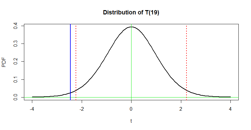
Suppose I have the following $n = 20$ observations sampled at random, as listed and summarized below:

x
 [1] 37.0 38.4 46.2 57.1 40.2 39.0 54.7 54.0 52.5 37.1
[11] 49.6 45.7 43.6 41.1 49.7 56.3 41.8 53.8 48.1 38.3
summary(x)
   Min. 1st Qu.  Median    Mean 3rd Qu.    Max. 
  37.00   39.90   45.95   46.21   52.83   57.10 
sd(x)
[1] 6.919454

I suppose that the population from which these data were randomly sampled is normal, and I want to test $H_0: \mu = 50$ against $H_a: \mu \ne 50,$ where $\mu$ is the population mean. The sample mean is $\bar X = 46.2,$ which is somewhat below $50.$ I use a t test to find out if $\bar X$ is 'significantly' different from $50.$

t.test(x, mu=50)

        One Sample t-test

data:  x
t = -2.4495, df = 19, p-value = 0.02417
alternative hypothesis: true mean is not equal to 50
95 percent confidence interval:
 42.9716 49.4484
sample estimates:
mean of x 
    46.21 

I want to do this test at the 5% level of significance. If $\mu$ really is $50,$ I want the probability of rejecting $H_0$ in favor of the alternative $H_a$ to be 5%.

The t statistic, $T = -2.4495$ above, is distributed according to Student's t distribution with degrees of freedom $\nu = n - 1 = 20 - 1 = 19.$ That distribution puts 95% of its probability between $\pm 2.228$ (vertical red dotted lines in the plot below). These are the upper and lower 'critical values'.

The R code below finds the upper critical value. You can also find this critical value in printed tables of Student's t distribution.

qt(.975, 10)
[1] 2.228139

The observed value of the t statistic, $T = -2.4495,$ shown in the plot as a vertical blue line, lies beyond the lower critical value. So we say that the null hypothesis $H_0$ is rejected at the 5% level of significance.

A second way to see that we reject $H_0$ at the 5% level is shown in the output from the t test above. If $H_0$ is true, then the probability $$P(|T| \ge -2.4495)= P(T \le -2.4495) + P(T \ge 2.4495) = 0.2417.$$ If $H_0$ is true, this is the probability that the $T$-statistic lies farther from 0 (in either direction) than the observed value $T = -2.4495.$ We know to reject $H_0$ at the 5% level of significance because the P-value is smaller than 0.05.

2 * pt(-2.4495, 19)
[1] 0.02417408

Generally speaking, there is not sufficient information in printed tables of Student's t distribution to find an exact P-value. So you will ordinarily have to rely on computer output (or results from a statistical calculator) to compute P-values.

Using p-values has one advantage. If I want to test the null hypothesis at the 1% level, I know that I cannot reject $H_0$ at the 1% level because the P-value exceed 0.01. (So it is not necessary to 'tell' a computer program what your level of significance is. Once you get the P-value you can test at any desired level of significance.)

Note: I was not surprised that the t test rejected the null hypothesis because I simulated the 20 observations in R, sampling from a normal distribution with $\mu = 47.$

set.seed(815)
x = round(rnorm(20, 47, 7),1)