Return to Answer

added 321 characters in body

Source Link

edited Sep 27, 2019 at 6:00

86.6k
6
115
304

Sidenote: In the special case that $K=0$ you can use

plot(x,y)
mod <- glm(y~x, family = gaussian(link = log), start = c(2,-0.01))
lines(x,exp(predict(mod)),col=2)

which models the observed parameter $y$ as

$$y = exp(X\beta) + \epsilon = exp(\beta_0) \cdot exp(\beta_1 \cdot x) + \epsilon$$

Sidenote: In the special case that $K=0$ you can use

plot(x,y)
mod <- glm(y~x, family = gaussian(link = log), start = c(2,-0.01))
lines(x,exp(predict(mod)),col=2)

which models the observed parameter $y$ as

$$y = exp(X\beta) + \epsilon = exp(\beta_0) \cdot exp(\beta_1 \cdot x) + \epsilon$$

Source Link

created Sep 26, 2019 at 14:16

Sextus Empiricus

86.6k
6
115
304

This question has relationships with several other questions

I have three additional remarks regarding some points in this question.

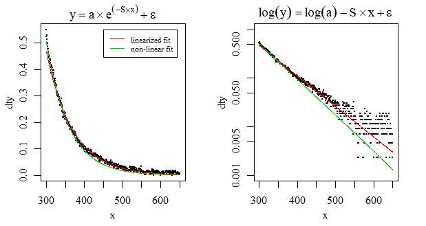
1: Why linearized model does not fit well the large values of $y$

Much better, but the model does not trace y values perfectly at low x values.

The linearized fit is not minimizing the same residuals. At the logarithmic scale the residuals for smaller values will be larger. The image below shows the comparison by plotting the y-axis on a log scale in the right image:

When necessary you could add weights to the least squares loss function.

2: Using linearized fit as starting values

After you have obtained estimates with your linearized fit you could have used these as starting point for the non linear fitting.*

# vectors x and y from data
x <- dat$x
y <- dat$y

# linearized fit with zero correction
K <- abs(min(y)) 
dty <- y + K*(1+10^-15)
fit <- lm(log(dty) ~x)  


# old fit that had a singluar gradient matrix error
#         nls(y ~ a * exp(-S * x) + K, 
#                 start = list(a = 0.5, 
#                              S = 0.1, 
#                              K = -0.1))
#

# new fit
fitnls <- nls(y ~ a * exp(-S * x) + K, 
                  start = list(a = exp(fit$coefficients[1]), 
                               S = -fit$coefficients[2], 
                               K = -0.1))
#

3: Using a more general method to obtain the starting point

If you have enough points then you can also obtain the slope without having to worry about asymptotic value and negative values (no computation of a logarithm needed).

You can do this by integrating the data points. Then with $$y = a e^{sx} + k $$ and $$Y = \frac{a}{s} e^{sx} + kx + Const$$ you can use a linear model to obtain the value of $s$ by describing $y$ as a linear combination of the vectors $Y$, $x$ and an intercept:

$$\begin{array}{rccccl}y &=& a e^{sx} + k &=& s(\frac{a}{s} e^{s x} + k x + Const) &- s k x - s Const \\ &&&=& sY &- sk x - s Const \end{array}$$

The advantage of this method (see Tittelbach and Helmrich 1993 "An integration method for the analysis of multiexponential transient signals") is that you can extend it to more than a single exponentially decaying component (adding more integrals).

#
# using Tittelbach Helmrich
#

# integrating with trapezium rule assuming x variable is already ordered
ys <- c(0,cumsum(0.5*diff(x)*(y[-1]+y[-length(y)])))

# getting slope parameter
modth <- lm(y ~ ys + x)
slope <- modth$coefficients[2]

# getting other parameters 
modlm <- lm(y ~ 1 + I(exp(slope*x)))
K <- modlm$coefficients[1]
a <- modlm$coefficients[2]

# fitting with TH start

fitnls2 <- nls(y ~ a * exp(-S * x) + K, 
              start = list(a = a, 
                           S = -slope, 
                           K = K))

Footnote: *This use of the slope in the linearized problem is exactly what what the SSasymp selfstarting function does. It first estimates the asymptote

> stats:::NLSstRtAsymptote.sortedXyData
function (xy) 
{
    in.range <- range(xy$y)
    last.dif <- abs(in.range - xy$y[nrow(xy)])
    if (match(min(last.dif), last.dif) == 2L) 
        in.range[2L] + diff(in.range)/8
    else in.range[1L] - diff(in.range)/8
}

and then the slope by (subtracting the asymptote value and taking the log values)

> stats:::NLSstAsymptotic.sortedXyData
function (xy) 
{
    xy$rt <- NLSstRtAsymptote(xy)
    setNames(coef(nls(y ~ cbind(1, 1 - exp(-exp(lrc) * x)), data = xy, 
        start = list(lrc = log(-coef(lm(log(abs(y - rt)) ~ x, 
            data = xy))[[2L]])), algorithm = "plinear"))[c(2, 
        3, 1)], c("b0", "b1", "lrc"))
}

Note the line start = list(lrc = log(-coef(lm(log(abs(y - rt)) ~ x, data = xy))[[2L]]))