Return to Answer

Since you do not give a model for the data I will describe one that has a similar look to your data and I belive it deals with the heteroscedasticity in a natural way.

Consider your observations $(X, Y)$ as a complex random variable such that $$ X + iY =Z e^{i (\theta + \varepsilon)}. $$

Where $Z$ and $\varepsilon$ are independendent real random variables with zero mean and finite variance and $\theta \in (-\pi/2 , \pi/2)$.

This model can be extended to include an unknown complex intercept which we omit for simplicity.

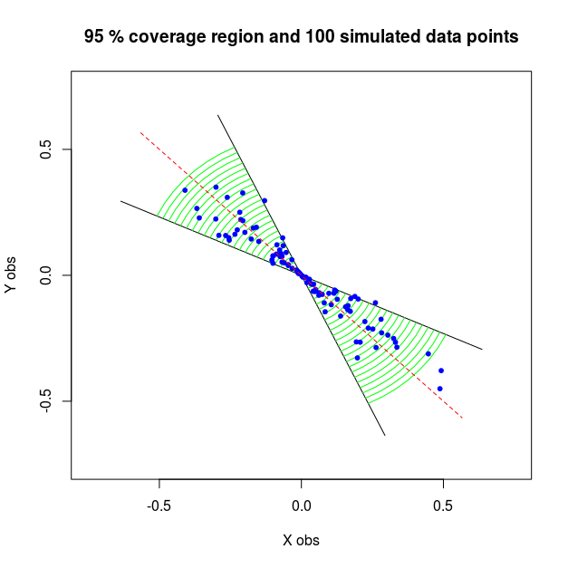
The following illustration shows a $\%95$ coverage region and a realization of 100 independet points with $\theta = -\pi/4$ and normaility for $Z$ and $\varepsilon$

$\%95$ coverage region " />

The idea of this model is that $\theta$ gives a line (red dashed in the figure) along which the process selects a point with $Z$ and then perturbates that point along the green lines by modifying it's phase by $\varepsilon$.

From the model definition we get that $$ \left. \begin{array}{1} Y = Z \sin (\theta + \varepsilon) \\ X = Z \cos (\theta + \varepsilon) \end{array} \right\} \implies Y = X \tan(\theta + \varepsilon) \implies \arctan(\frac{Y}{X}) = \theta +\varepsilon. $$ From a sample $(X_1, Y_1) \ldots (X_n,Y_n)$ we get the following estimation $$ \hat \theta = \frac{1}{n} \sum_{k = 1}^n \arctan (\frac{Y_k}{X_k})$$

From a new observation $X_{new}$ we can construct a a new value $$Y_{new} = X_{new}\tan( \hat \theta )$$

It is important to note that the least squares estimatior derived from the model $$Y = X \beta + \varepsilon, $$ is different from the one we obtained.

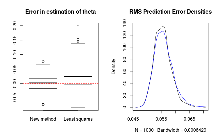
This is made explicit in the following figure where the boxplot shows the error for estimating $\theta$ with $\hat \theta$ and $\arctan(\hat \beta)$ . It was obtained with 1000 replications under the same scenario as the first figure with $n = 40$ samples. The least squares estimator is clearly biased and has higher variability.

The second plot in the figure compares the densities of the Root Mean squared Prediction Error for both methods. After each of the 1000 estimation 1000 new points were independently generated. The blue line corresponds to the least squares method. It is clear that at least in this scenario the described method is superior also in prediction.

Finally note that taking logs to obtain a linear model is not so easy because $Y$ and $X$ can have different sign.

Since you do not give a model I will describe one that has a similar look to your data and I belive it deals with the heteroscedasticity in a natural way.

Consider your observations $(X, Y)$ as a complex random variable such that $$ X + iY =Z e^{i (\theta + \varepsilon)}. $$

Where $Z$ and $\varepsilon$ are independendent real random variables with zero mean and finite variance and $\theta \in (-\pi/2 , \pi/2)$.

This model can be extended to include an unknown complex intercept which we omit for simplicity.

The following illustration shows a $\%95$ coverage region and a realization of 100 independet points with $\theta = -\pi/4$ and normaility for $Z$ and $\varepsilon$

$\%95$ coverage region " />

The idea of this model is that $\theta$ gives a line (red dashed in the figure) along which the process selects a point with $Z$ and then perturbates that point along the green lines by modifying it's phase by $\varepsilon$.

From the model definition we get that $$ \left. \begin{array}{1} Y = Z \sin (\theta + \varepsilon) \\ X = Z \cos (\theta + \varepsilon) \end{array} \right\} \implies Y = X \tan(\theta + \varepsilon) \implies \arctan(\frac{Y}{X}) = \theta +\varepsilon. $$ From a sample $(X_1, Y_1) \ldots (X_n,Y_n)$ we get the following estimation $$ \hat \theta = \frac{1}{n} \sum_{k = 1}^n \arctan (\frac{Y_k}{X_k})$$

From a new observation $X_{new}$ we can construct a a new value $$Y_{new} = X_{new}\tan( \hat \theta )$$

It is important to note that the least squares estimatior derived from the model $$Y = X \beta + \varepsilon, $$ is different from the one we obtained.

This is made explicit in the following figure where the boxplot shows the error for estimating $\theta$ with $\hat \theta$ and $\arctan(\hat \beta)$ . It was obtained with 1000 replications under the same scenario as the first figure with $n = 40$ samples. The least squares estimator is clearly biased and has higher variability.

The second plot in the figure compares the densities of the Root Mean squared Prediction Error for both methods. After each of the 1000 estimation 1000 new points were independently generated. The blue line corresponds to the least squares method. It is clear that at least in this scenario the described method is superior also in prediction.

Since you do not give a model for the data I will describe one that has a similar look to your data and I belive it deals with the heteroscedasticity in a natural way.

Consider your observations $(X, Y)$ as a complex random variable such that $$ X + iY =Z e^{i (\theta + \varepsilon)}. $$

Where $Z$ and $\varepsilon$ are independendent real random variables with zero mean and finite variance and $\theta \in (-\pi/2 , \pi/2)$.

This model can be extended to include an unknown complex intercept which we omit for simplicity.

The following illustration shows a $\%95$ coverage region and a realization of 100 independet points with $\theta = -\pi/4$ and normaility for $Z$ and $\varepsilon$

$\%95$ coverage region " />

The idea of this model is that $\theta$ gives a line (red dashed in the figure) along which the process selects a point with $Z$ and then perturbates that point along the green lines by modifying it's phase by $\varepsilon$.

From the model definition we get that $$ \left. \begin{array}{1} Y = Z \sin (\theta + \varepsilon) \\ X = Z \cos (\theta + \varepsilon) \end{array} \right\} \implies Y = X \tan(\theta + \varepsilon) \implies \arctan(\frac{Y}{X}) = \theta +\varepsilon. $$ From a sample $(X_1, Y_1) \ldots (X_n,Y_n)$ we get the following estimation $$ \hat \theta = \frac{1}{n} \sum_{k = 1}^n \arctan (\frac{Y_k}{X_k})$$

From a new observation $X_{new}$ we can construct a a new value $$Y_{new} = X_{new}\tan( \hat \theta )$$

It is important to note that the least squares estimatior derived from the model $$Y = X \beta + \varepsilon, $$ is different from the one we obtained.

This is made explicit in the following figure where the boxplot shows the error for estimating $\theta$ with $\hat \theta$ and $\arctan(\hat \beta)$ . It was obtained with 1000 replications under the same scenario as the first figure with $n = 40$ samples. The least squares estimator is clearly biased and has higher variability.

The second plot in the figure compares the densities of the Root Mean squared Prediction Error for both methods. After each of the 1000 estimation 1000 new points where independently generated. The blue line corresponds to the least squares method. It is clear that at least in this scenario the described method is superior also in prediction.

Finally note that taking logs to obtain a linear model is not so easy because $Y$ and $X$ can have different sign.

Since you do not give a model for the data I will describe one that has a similar look to your data and I belive it deals with the heteroscedasticity in a natural way.

Consider your observations $(X, Y)$ as a complex random variable such that $$ X + iY =Z e^{i (\theta + \varepsilon)}. $$

Where $Z$ and $\varepsilon$ are independendent real random variables with zero mean and finite variance and $\theta \in (-\pi/2 , \pi/2)$.

This model can be extended to include an unknown complex intercept which we omit for simplicity.

The following illustration shows a $\%95$ coverage region and a realization of 100 independet points with $\theta = -\pi/4$ and normaility for $Z$ and $\varepsilon$

$\%95$ coverage region " />

The idea of this model is that $\theta$ gives a line (red dashed in the figure) along which the process selects a point with $Z$ and then perturbates that point along the green lines by modifying it's phase by $\varepsilon$.

From the model definition we get that $$ \left. \begin{array}{1} Y = Z \sin (\theta + \varepsilon) \\ X = Z \cos (\theta + \varepsilon) \end{array} \right\} \implies Y = X \tan(\theta + \varepsilon) \implies \arctan(\frac{Y}{X}) = \theta +\varepsilon. $$ From a sample $(X_1, Y_1) \ldots (X_n,Y_n)$ we get the following estimation $$ \hat \theta = \frac{1}{n} \sum_{k = 1}^n \arctan (\frac{Y_k}{X_k})$$

From a new observation $X_{new}$ we can construct a a new value $$Y_{new} = X_{new}\tan( \hat \theta )$$

It is important to note that the least squares estimatior derived from the model $$Y = X \beta + \varepsilon, $$ is different from the one we obtained.

This is made explicit in the following figure where the boxplot shows the error for estimating $\theta$ with $\hat \theta$ and $\arctan(\hat \beta)$ . It was obtained with 1000 replications under the same scenario as the first figure with $n = 40$ samples. The least squares estimator is clearly biased and has higher variability.

The second plot in the figure compares the densities of the Root Mean squared Prediction Error for both methods. After each of the 1000 estimation 1000 new points were independently generated. The blue line corresponds to the least squares method. It is clear that at least in this scenario the described method is superior also in prediction.

Finally note that taking logs to obtain a linear model is not so easy because $Y$ and $X$ can have different sign.

Since you do not give a model for the data I will describe one that has a similar look to your data and I belive it deals with the heteroscedasticity in a natural way.

Consider your observations $(X, Y)$ as a complex random variable such that $$ X + iY =Z e^{i (\theta + \varepsilon)}. $$

Where $Z$ and $\varepsilon$ are independendent real random variables with zero mean and finite variance and $\theta \in (-\pi/2 , \pi/2)$.

This model can be extended to include an unknown complex intercept which we omit for simplicity.

The following illustration shows a $\%95$ coverage region and a realization of 100 independet points with $\theta = -\pi/4$ and normaility for $Z$ and $\varepsilon$

$\%95$ coverage region " />

The idea of this model is that $\theta$ gives a line (red dashed in the figure) along which the process selects a point with $Z$ and then perturbates that point along the green lines by modifying it's phase by $\varepsilon$.

From the model definition we get that $$ \left. \begin{array}{1} Y = Z \sin (\theta + \varepsilon) \\ X = Z \cos (\theta + \varepsilon) \end{array} \right\} \implies Y = X \tan(\theta + \varepsilon) \implies \arctan(\frac{Y}{X}) = \theta +\varepsilon. $$ From a sample $(X_1, Y_1) \ldots (X_n,Y_n)$ we get the following estimation $$ \hat \theta = \frac{1}{n} \sum_{k = 1}^n \arctan (\frac{Y_k}{X_k})$$

From a new observation $X_{new}$ we can construct a a new value $$Y_{new} = X_{new}\tan( \hat \theta )$$

It is important to note that the least squares estimatior derived from the model $$Y = X \beta + \varepsilon, $$ is different from the one we obtained.

This is made explicit in the following figure where the boxplot shows the error for estimating $\theta$ with $\hat \theta$ and $\arctan(\hat \beta)$ . It was obtained with 1000 replications under the same scenario as the first figure with $n = 40$ samples. The least squares estimator is clearly biased and has higher variability.

The second plot in the figure compares the densities of the Root Mean squared Prediction Error for both methods. After each of the 1000 estimation 1000 new points where independently generated. The blue line corresponds to the least squares method. It is clear that at least in this scenario the described method is superior also in prediction.

Finally note that taking logs to obtain a linear model is not so easy because $Y$ and $X$ can have different signs.

Since you do not give a model for the data I will describe one that has a similar look to your data and I belive it deals with the heteroscedasticity in a natural way.

Consider your observations $(X, Y)$ as a complex random variable such that $$ X + iY =Z e^{i (\theta + \varepsilon)}. $$

Where $Z$ and $\varepsilon$ are independendent real random variables with zero mean and finite variance and $\theta \in (-\pi/2 , \pi/2)$.

This model can be extended to include an unknown complex intercept which we omit for simplicity.

The following illustration shows a $\%95$ coverage region and a realization of 100 independet points with $\theta = -\pi/4$ and normaility for $Z$ and $\varepsilon$

$\%95$ coverage region " />

The idea of this model is that $\theta$ gives a line (red dashed in the figure) along which the process selects a point with $Z$ and then perturbates that point along the green lines by modifying it's phase by $\varepsilon$.

From the model definition we get that $$ \left. \begin{array}{1} Y = Z \sin (\theta + \varepsilon) \\ X = Z \cos (\theta + \varepsilon) \end{array} \right\} \implies Y = X \tan(\theta + \varepsilon) \implies \arctan(\frac{Y}{X}) = \theta +\varepsilon. $$ From a sample $(X_1, Y_1) \ldots (X_n,Y_n)$ we get the following estimation $$ \hat \theta = \frac{1}{n} \sum_{k = 1}^n \arctan (\frac{Y_k}{X_k})$$

From a new observation $X_{new}$ we can construct a a new value $$Y_{new} = X_{new}\tan( \hat \theta )$$

It is important to note that the least squares estimatior derived from the model $$Y = X \beta + \varepsilon, $$ is different from the one we obtained.

This is made explicit in the following figure where the boxplot shows the error for estimating $\theta$ with $\hat \theta$ and $\arctan(\hat \beta)$ . It was obtained with 1000 replications under the same scenario as the first figure with $n = 40$ samples. The least squares estimator is clearly biased and has higher variability.

The second plot in the figure compares the densities of the Root Mean squared Prediction Error for both methods. After each of the 1000 estimation 1000 new points where independently generated. The blue line corresponds to the least squares method. It is clear that at least in this scenario the described method is superior also in prediction.

Finally note that taking logs to obtain a linear model is not so easy because $Y$ and $X$ can have different sign.