added 148 characters in body
Source Link
BruceET
  • 57.6k
  • 2
  • 36
  • 94

The number $X$ of 6's in 4 trials has $X \sim \mathsf{Binom}(n=4,p=1/6)$ and he number $Y$ of 6's in 8 trials has $Y \sim \mathsf{Binom}(n=8,p=1/6).$

In R, $P(X \ge 1) = 1 - P(X = 0) = 0.5177.$

1-dbinom(0, 4, 1/6)
[1] 0.5177469

By contrast, $P(Y \ge 2) = 1 - P(X \le 1) = 0.3953,$ smaller than above.

1 - pbinom(1, 8, 1/6)
[1] 0.3953231

By simulation of a million games of each type:

set.seed(1120)
x = replicate(10^6,  sum(sample(1:6, 4, rep=T)==6))
mean(x >= 1)
[1] 0.517721     # aprx 0.5177

y = replicate(10^6,  sum(sample(1:6, 8, rep=T)==6))
mean(y >= 2)
[1] 0.395072      # aprx 0.3953 +/- 0.001
2*sd(y >= 2)/1000
[1] 0.0009777328  # 95% margin of simulation error

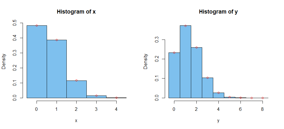
In each figure below, the histogram summarizes simulated values and the (centers of) red circles show exact binomial probabilities.

enter image description here

par(mfrow=c(1,2))
 hist(x, prob=T, br = (-1:4)+.5, col="skyblue2")
  points(0:4, dbinom(0:4, 4, 1/6), col="red")
 hist(y, prob=T, br = (-1:8)+.5, col="skyblue2")
  points(0:8, dbinom(0:8, 8, 1/6), col="red")
par(mfrow=c(1,1))

Bottom line: There are only $625$ chances in $1296$ to lose the first game and $1\,015\,625$ chances in $1\,679\,616$ to lose the second.

The number $X$ of 6's in 4 trials has $X \sim \mathsf{Binom}(n=4,p=1/6)$ and he number $Y$ of 6's in 8 trials has $Y \sim \mathsf{Binom}(n=8,p=1/6).$

In R, $P(X \ge 1) = 1 - P(X = 0) = 0.5177.$

1-dbinom(0, 4, 1/6)
[1] 0.5177469

By contrast, $P(Y \ge 2) = 1 - P(X \le 1) = 0.3953,$ smaller than above.

1 - pbinom(1, 8, 1/6)
[1] 0.3953231

By simulation of a million games of each type:

set.seed(1120)
x = replicate(10^6,  sum(sample(1:6, 4, rep=T)==6))
mean(x >= 1)
[1] 0.517721     # aprx 0.5177

y = replicate(10^6,  sum(sample(1:6, 8, rep=T)==6))
mean(y >= 2)
[1] 0.395072      # aprx 0.3953 +/- 0.001
2*sd(y >= 2)/1000
[1] 0.0009777328  # 95% margin of simulation error

In each figure below, the histogram summarizes simulated values and the (centers of) red circles show exact binomial probabilities.

enter image description here

par(mfrow=c(1,2))
 hist(x, prob=T, br = (-1:4)+.5, col="skyblue2")
  points(0:4, dbinom(0:4, 4, 1/6), col="red")
 hist(y, prob=T, br = (-1:8)+.5, col="skyblue2")
  points(0:8, dbinom(0:8, 8, 1/6), col="red")
par(mfrow=c(1,1))

Bottom line: There are only $625$ chances in $1296$ to lose the first game and $1\,015\,625$ chances in $1\,679\,616$ to lose the second.

added 486 characters in body
Source Link
BruceET
  • 57.6k
  • 2
  • 36
  • 94

The number $X$ of 6's in 4 trials has $X \sim \mathsf{Binom}(n=4,p=1/6)$ and he number $Y$ of 6's in 8 trials has $Y \sim \mathsf{Binom}(n=8,p=1/6).$

In R, $P(X \ge 1) = 1 - P(X = 0) = 0.5177.$

1-dbinom(0, 4, 1/6)
[1] 0.5177469

By contrast, $P(Y \ge 2) = 1 - P(X \le 1) = 0.3953,$ smaller than above.

1 - pbinom(1, 8, 1/6)
[1] 0.3953231

By simulation of a million games of each type:

set.seed(1120)
x = replicate(10^6,  sum(sample(1:6, 4, rep=T)==6))
mean(x >= 1)
[1] 0.517721     # aprx 0.5177

y = replicate(10^6,  sum(sample(1:6, 8, rep=T)==6))
mean(y >= 2)
[1] 0.395072      # aprx 0.3953 +/- 0.001
2*sd(y >= 2)/1000
[1] 0.0009777328  # 95% margin of simulation error

In each figure below, the histogram summarizes simulated values and the (centers of) red circles show exact binomial probabilities.

enter image description here

par(mfrow=c(1,2))
 hist(x, prob=T, br = (-1:4)+.5, col="skyblue2")
  points(0:4, dbinom(0:4, 4, 1/6), col="red")
 hist(y, prob=T, br = (-1:8)+.5, col="skyblue2")
  points(0:8, dbinom(0:8, 8, 1/6), col="red")
par(mfrow=c(1,1))

The number $X$ of 6's in 4 trials has $X \sim \mathsf{Binom}(n=4,p=1/6)$ and he number $Y$ of 6's in 8 trials has $Y \sim \mathsf{Binom}(n=8,p=1/6).$

In R, $P(X \ge 1) = 1 - P(X = 0) = 0.5177.$

1-dbinom(0, 4, 1/6)
[1] 0.5177469

By contrast, $P(Y \ge 2) = 1 - P(X \le 1) = 0.3953,$ smaller than above.

1 - pbinom(1, 8, 1/6)
[1] 0.3953231

By simulation of a million games of each type:

set.seed(1120)
x = replicate(10^6,  sum(sample(1:6, 4, rep=T)==6))
mean(x >= 1)
[1] 0.517721     # aprx 0.5177

y = replicate(10^6,  sum(sample(1:6, 8, rep=T)==6))
mean(y >= 2)
[1] 0.395072      # aprx 0.3953 +/- 0.001
2*sd(y >= 2)/1000
[1] 0.0009777328  # 95% margin of simulation error

In each figure below, the histogram summarizes simulated values and the (centers of) red circles show exact binomial probabilities.

enter image description here

par(mfrow=c(1,2))
 hist(x, prob=T, br = (-1:4)+.5, col="skyblue2")
  points(0:4, dbinom(0:4, 4, 1/6), col="red")
 hist(y, prob=T, br = (-1:8)+.5, col="skyblue2")
  points(0:8, dbinom(0:8, 8, 1/6), col="red")
par(mfrow=c(1,1))
Source Link
BruceET
  • 57.6k
  • 2
  • 36
  • 94

The number $X$ of 6's in 4 trials has $X \sim \mathsf{Binom}(n=4,p=1/6)$ and he number $Y$ of 6's in 8 trials has $Y \sim \mathsf{Binom}(n=8,p=1/6).$

In R, $P(X \ge 1) = 1 - P(X = 0) = 0.5177.$

1-dbinom(0, 4, 1/6)
[1] 0.5177469

By contrast, $P(Y \ge 2) = 1 - P(X \le 1) = 0.3953,$ smaller than above.

1 - pbinom(1, 8, 1/6)
[1] 0.3953231

By simulation of a million games of each type:

set.seed(1120)
x = replicate(10^6,  sum(sample(1:6, 4, rep=T)==6))
mean(x >= 1)
[1] 0.517721     # aprx 0.5177

y = replicate(10^6,  sum(sample(1:6, 8, rep=T)==6))
mean(y >= 2)
[1] 0.395072      # aprx 0.3953 +/- 0.001
2*sd(y >= 2)/1000
[1] 0.0009777328  # 95% margin of simulation error