added 3772 characters in body
Source Link
tchakravarty
  • 9k
  • 2
  • 42
  • 55

Update to follow-up

Let me rewrite your model one more time $$ Y_i = \beta_0 + \beta_1Z_{1i} + \beta_2 Z_{2i} + \beta_3 X_i + U_{1i} $$ where as before, $Z_{1i}$ and $Z_{2i}$ are exogenous and $X_i$ is endogenous. You assume the data generating process $$ \begin{align} Z_{2i} &= \mathbf{1}_{[i\text{ is odd}]}\\ X_i &= \alpha_0 + \alpha_1Z_{1i} + U_{2i} \end{align} $$ You introduce endogeneity by assuming that $U_{1i}$ and $U_{2i}$ are correlated. $$ \mathbb{C}(U_{1i}, U_{2i}) = \rho $$

Also, you assume that the errors in the reduced form equation are heteroskedastic: $$ \begin{align} \mathbb{V}(U_{2i}\mid Z_{2i} = 0) &= 1 \\ \mathbb{V}(U_{2i}\mid Z_{2i} = 1) &= \tfrac{1}{q} \\ \end{align} $$

Here is the Stata code to simulate this DGP.

clear*
program simcont, rclass
    syntax [, Q(real 1.0)]

    drop _all
    set obs 1000
    scalar beta0 = 5
    scalar beta1 = 1
    scalar beta2 = 2
    scalar beta3 = 3

    scalar alpha0 = 1
    scalar alpha1 = 4

    scalar rho = 0.1

    g z1 = rnormal()
    g z2 = mod(_n, 2)
    scalar a11 = 1
    scalar a12 = rho*sqrt(1)*sqrt(1)
    scalar a13 = rho*sqrt(1)*sqrt(1/`q')
    scalar a21 = rho*sqrt(1)*sqrt(1)
    scalar a22 = 1
    scalar a23 = 0
    scalar a31 = rho*sqrt(1)*sqrt(1/`q')
    scalar a32 = 0
    scalar a33 = 1/`q'

    mat corrMatrix= (a11, a12, a13 \ a21, a22, a23 \a31, a32, a33)
    drawnorm u1 u3 u4, cov(corrMatrix)
    g u2 = cond(z2, u3, u4)

    g x = alpha0 + alpha1*z2 + u2
    g y = beta0 + beta1*z1 + beta2*z2 + beta3*x + u1
    reg y z1 z2 x
    mat mA = e(b)
    return scalar ols = el(mA, 1, colnumb(mA, "x"))
    
    // return the results of the heteroskedasticity test
    qui reg x z2
    estat hettest, rhs iid
    return scalar hettestPValues = r(p)
end

// simulate to check for heteroskedasticity
simulate olsCoeff = r(ols) hettestPValues = r(hettestPValues), reps(100): simcont, q(5) 
su hettestPValues // strong evidence of heteroskedasticity in the reduced form

cap mat drop biasBeta
forvalues q = 2(1)5 {
    simulate olsCoeff = r(ols), reps(1000): simcont, q(`q') 
    qui su olsCoeff
    mat biasBeta = (nullmat(biasBeta), r(mean) - 3)
    local colNames "`colNames' q:`q' "
}
mat colnames biasBeta = `colNames'
mat list biasBeta
  • Note that the heteroskedasticity is where you put it in the model, and the simulation results are now able to find it.
. su hettestPValues // strong evidence of heteroskedasticity in the reduced form

    Variable |       Obs        Mean    Std. Dev.       Min        Max
-------------+--------------------------------------------------------
hettestPVa~s |       100    1.53e-26    8.12e-26   3.09e-38   6.22e-25
  • Also, I can confirm that what you claim is actually true, that as the heteroskedasticity in the reduced form equation increases, the bias in the OLS estimator also increases.
biasBeta[1,4]
            q:         q:         q:         q:
            2          3          4          5
r1  .11242463  .11808594  .12122701  .12210455

A simple explanation of this is that as $q$ increases, the conditional (on $Z_{2i}=1$) and hence the unconditional variance of the reduced form error $U_{2i}$ decreases (check through a variance decomposition) which means that the variance of the endogenous regressor decreases, which means that the $(\mathbf{X}'\mathbf{X})^{-1}$ increases in magnitude, and the overall bias increases (this is a very rough description -- I am sure it can be formalized).

added 3172 characters in body
Source Link
tchakravarty
  • 9k
  • 2
  • 42
  • 55

Follow-up questions:

The OP has asked for some clarifications in the comments for which I am providing an updated answer.

Let me rewrite your model $$ Y_i = \beta_0 + \beta_1 Z_{1i} + \beta_2 Z_{2i} + \beta_3 X_i + U_i $$ where $Z_{1i}$ and $Z_{2i}$ are exogenous, and $X_{i}$ is endogenous, that is $\mathbb{E}(X_iU_i) = \rho$. In addition, you want the variable $Z_{2i}$ to be constructed as $$ Z_{2i} = \mathbf{1}_{[i\text{ is odd.}]} $$ You are simulating the OLS estimates of the coefficient on $X_i$, that is $\beta_3$. Here is a small Stata script to do that.

clear*
program simcont, rclass
    syntax [, errorVariance(real 1.0)]
    drop _all
    set obs 1000
    scalar beta0 = 5
    scalar beta1 = 1
    scalar beta2 = 2
    scalar beta3 = 3
    scalar rho = 0.1

    g z1 = rnormal()
    g z2 = mod(_n, 2)
    g u = sqrt(`errorVariance')*rnormal() 
    g x = rho*u/`errorVariance' + rnormal()

    g y = beta0 + beta1*z1 + beta2*z2 + beta3*x + u
    reg y z1 z2 x
    mat mA = e(b)
    return scalar ols = el(mA, 1, colnumb(mA, "x"))
    
    // return the results of the heteroskedasticity test
    estat hettest, rhs iid
    return scalar hettestPValues = r(p)
end

// simulate with error variance = 1
simulate olsCoeff = r(ols) hettestPValues = r(hettestPValues), reps(100): simcont 
su olsCoeff hettestPValues // p-values have the correct mean; no heteroskedasticity

cap mat drop biasBeta
forvalues errorVariance = 2(1)6 {
    simulate olsCoeff = r(ols), reps(100): simcont, errorVariance(`errorVariance') 
    qui su olsCoeff
    mat biasBeta = (nullmat(biasBeta), r(mean) - 3)
    local colNames "`colNames' errVar:`errorVariance' "
}
mat colnames biasBeta = `colNames'
mat list biasBeta

Now note that there are at least two discrepancies here.

  • The first thing is that there is no heteroskedasticity in the model as you have written it. The mean of the p-values of an LM test of homoskedasticity from the simulations indicates that they are being drawn under the null.
. su olsCoeff hettestPValues // p-values have the correct mean; no heteroskedasticity

    Variable |       Obs        Mean    Std. Dev.       Min        Max
-------------+--------------------------------------------------------
    olsCoeff |       100    3.094182    .0326048   3.007202   3.179945
hettestPVa~s |       100    .4762952    .2885692   .0039824   .9844939
  • The next thing to note is that the bias is that the asymptotic bias is the same for all values of the error variance, as long as the degree of endogeneity is the same. Here are the results of my simulation
. mat list biasBeta

biasBeta[1,5]
       errVar:    errVar:    errVar:    errVar:    errVar:
            2          3          4          5          6
r1  .09913641  .10274499   .0912232  .11309942  .09122764

If you are getting results different than this, then you should show us your code, and we can compare the two.

Bounty Ended with 50 reputation awarded by Druss2k
Source Link
tchakravarty
  • 9k
  • 2
  • 42
  • 55

While this is not a situation that arises in practice, this is related to the so-called control function approach to dealing with endogeneity.

Let me rewrite your (simple) model $$ Y_i = \beta_0 + \beta_1X_i + U_i $$ together with your assumptions $\mathbb{E}(U_i)=0$ and $\mathbb{E}(U_iX_i)=\rho$.

Then $$ \mathbb{E}(X_i(U_i-\frac{\rho}{X_i}))=0 $$ so that if I rewrite my model $$ Y_i = \beta_0 + \beta_1X_i + \frac{\rho}{X_i} + \underbrace{U_i-\frac{\rho}{X_i}}_{\equiv V_i} $$ and estimate this model by OLS, constraining the coefficient of the $\frac{1}{X_i}$ term to be $\rho$, I should get consistent estimates of $\beta_1$.


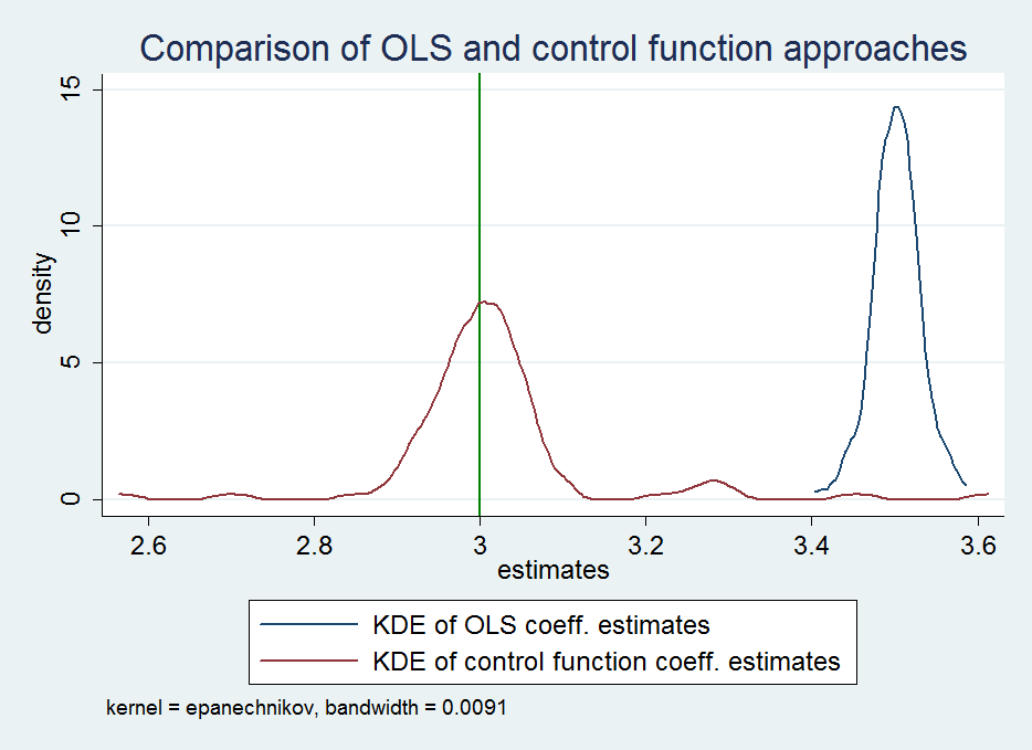
So, consider the following Stata simulations

clear*
program simcont, rclass
    drop _all
    set obs 1000
    g x1 = rnormal()
    g x2 = rnormal()
    g u = x1 + rnormal()
    g x = x1 + x2
    
    g y = 2 + 3*x + u  // ols 
    reg y x
    mat mA = e(b)
    return scalar ols = el(mA, 1, colnumb(mA, "x"))
    
    g cont = 1/x
    constraint define 1 cont = 1  // true correlation between error and regressor
    cnsreg y x cont, constraints(1)  // constrained regression
    mat mA = e(b)
    return scalar cont = el(mA, 1, colnumb(mA, "x"))
end

simulate olsCoeff = r(ols) controlFuncCoeff=r(cont), reps(100): simcont 

kdensity olsCoeff, xline(3, lcolor(green)) addplot(kdensity controlFuncCoeff) ///
    legend(label(1 "KDE of OLS coeff. estimates") label(2 "KDE of control function coeff. estimates")) ///
    xtitle("estimates") ytitle("density") title("Comparison of OLS and control function approaches") 

which produces the following picture (based on 100 replications)

enter image description here

However, I would think very carefully and experiment with more regressors and in general more data configurations before I put this estimation strategy to work on real data.