added 1 character in body
Source Link
whuber
  • 333.6k
  • 63
  • 792
  • 1.3k

The lesson of extreme value theorylesson of extreme value theory is that when you rescale the maximum of $m$ iid standard Normal variables by an amount proportional to $\sqrt{2\log m}$ and shift that to a location near $\sqrt{2\log m},$ it converges to the standard Gumbel distribution as $m$ increases.

If first you rescale your $m$ iid Normal variables by $\sqrt{m},$ they become standard Normal, and the preceding applies.

Consequently, for suitable constants $\alpha$ and $\beta,$ $$Z_m \beta \sqrt{2m\log m} - \alpha \sqrt{2\log m}$$ converges to a Gumbel distribution.

In particular, this means we may approximate $Z_m$ closely (in distribution) by

$$Z_m \approx \frac{Y }{\beta \sqrt{2m\log m}} + \frac{\alpha}{\beta\sqrt{m}}$$

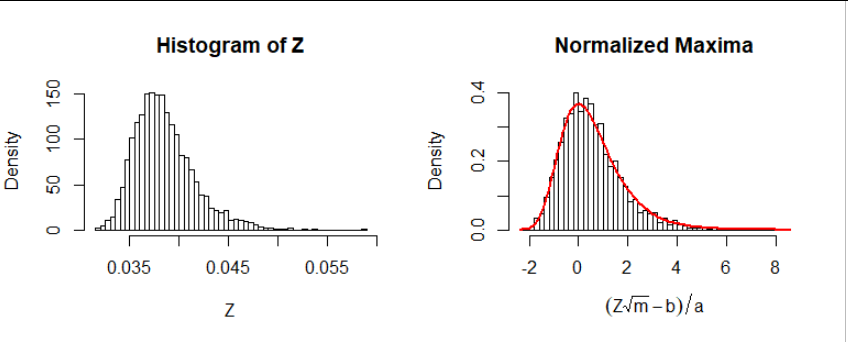
for a Gumbel variate $Y.$ Since the denominators diverge, the (unnormalized) limiting distribution of $Z_m$ is $0$ (in probability). Notice that it does so by being squeezed narrowly around a positive value $\alpha / (\beta\sqrt{m})$ while this central value creeps slowly down towards zero. Here's a histogram with $m=10000$ based on $4000$ such samples:

Figure

The red curve plots the limiting Gumbel density, $f(y) = \exp(-e^{-y} - y).$

The lesson of extreme value theory is that when you rescale the maximum of $m$ iid standard Normal variables by an amount proportional to $\sqrt{2\log m}$ and shift that to a location near $\sqrt{2\log m},$ it converges to the standard Gumbel distribution as $m$ increases.

If first you rescale your $m$ iid Normal variables by $\sqrt{m},$ they become standard Normal, and the preceding applies.

Consequently, for suitable constants $\alpha$ and $\beta,$ $$Z_m \beta \sqrt{2m\log m} - \alpha \sqrt{2\log m}$$ converges to a Gumbel distribution.

In particular, this means we may approximate $Z_m$ closely (in distribution) by

$$Z_m \approx \frac{Y }{\beta \sqrt{2m\log m}} + \frac{\alpha}{\beta\sqrt{m}}$$

for a Gumbel variate $Y.$ Since the denominators diverge, the (unnormalized) limiting distribution of $Z_m$ is $0$ (in probability). Notice that it does so by being squeezed narrowly around a positive value $\alpha / (\beta\sqrt{m})$ while this central value creeps slowly down towards zero. Here's a histogram with $m=10000$ based on $4000$ such samples:

Figure

The red curve plots the limiting Gumbel density, $f(y) = \exp(-e^{-y} - y).$
The lesson of extreme value theory is that when you rescale the maximum of $m$ iid standard Normal variables by an amount proportional to $\sqrt{2\log m}$ and shift that to a location near $\sqrt{2\log m},$ it converges to the standard Gumbel distribution as $m$ increases.

If first you rescale your $m$ iid Normal variables by $\sqrt{m},$ they become standard Normal, and the preceding applies.

Consequently, for suitable constants $\alpha$ and $\beta,$ $$Z_m \beta \sqrt{2m\log m} - \alpha \sqrt{2\log m}$$ converges to a Gumbel distribution.

In particular, this means we may approximate $Z_m$ closely (in distribution) by

$$Z_m \approx \frac{Y }{\beta \sqrt{2m\log m}} + \frac{\alpha}{\beta\sqrt{m}}$$

for a Gumbel variate $Y.$ Since the denominators diverge, the (unnormalized) limiting distribution of $Z_m$ is $0$ (in probability). Notice that it does so by being squeezed narrowly around a positive value $\alpha / (\beta\sqrt{m})$ while this central value creeps slowly down towards zero. Here's a histogram with $m=10000$ based on $4000$ such samples:

Figure

The red curve plots the limiting Gumbel density, $f(y) = \exp(-e^{-y} - y).$

remove misleading closing parenthese ")"
Source Link
Yves
  • 5.7k
  • 1
  • 23
  • 38

The lesson of extreme value theory is that when you rescale the maximum of $m$ iid standard Normal variables by an amount proportional to $\sqrt{2\log m}$ and shift that to a location near $\sqrt{2\log m},$ it converges to the standard Gumbel distribution as $m$ increases.

If first you rescale your $m$ iid Normal variables by $\sqrt{m},$ they become standard Normal, and the preceding applies.

Consequently, for suitable constants $\alpha$ and $\beta,$ $$Z_m \beta \sqrt{2m\log m}) - \alpha \sqrt{2\log m}$$$$Z_m \beta \sqrt{2m\log m} - \alpha \sqrt{2\log m}$$ converges to a Gumbel distribution.

In particular, this means we may approximate $Z_m$ closely (in distribution) by

$$Z_m \approx \frac{Y }{\beta \sqrt{2m\log m}} + \frac{\alpha}{\beta\sqrt{m}}$$

for a Gumbel variate $Y.$ Since the denominators diverge, the (unnormalized) limiting distribution of $Z_m$ is $0$ (in probability). Notice that it does so by being squeezed narrowly around a positive value $\alpha / (\beta\sqrt{m})$ while this central value creeps slowly down towards zero. Here's a histogram with $m=10000$ based on $4000$ such samples:

Figure

The red curve plots the limiting Gumbel density, $f(y) = \exp(-e^{-y} - y).$

The lesson of extreme value theory is that when you rescale the maximum of $m$ iid standard Normal variables by an amount proportional to $\sqrt{2\log m}$ and shift that to a location near $\sqrt{2\log m},$ it converges to the standard Gumbel distribution as $m$ increases.

If first you rescale your $m$ iid Normal variables by $\sqrt{m},$ they become standard Normal, and the preceding applies.

Consequently, for suitable constants $\alpha$ and $\beta,$ $$Z_m \beta \sqrt{2m\log m}) - \alpha \sqrt{2\log m}$$ converges to a Gumbel distribution.

In particular, this means we may approximate $Z_m$ closely (in distribution) by

$$Z_m \approx \frac{Y }{\beta \sqrt{2m\log m}} + \frac{\alpha}{\beta\sqrt{m}}$$

for a Gumbel variate $Y.$ Since the denominators diverge, the (unnormalized) limiting distribution of $Z_m$ is $0$ (in probability). Notice that it does so by being squeezed narrowly around a positive value $\alpha / (\beta\sqrt{m})$ while this central value creeps slowly down towards zero. Here's a histogram with $m=10000$ based on $4000$ such samples:

Figure

The red curve plots the limiting Gumbel density, $f(y) = \exp(-e^{-y} - y).$

The lesson of extreme value theory is that when you rescale the maximum of $m$ iid standard Normal variables by an amount proportional to $\sqrt{2\log m}$ and shift that to a location near $\sqrt{2\log m},$ it converges to the standard Gumbel distribution as $m$ increases.

If first you rescale your $m$ iid Normal variables by $\sqrt{m},$ they become standard Normal, and the preceding applies.

Consequently, for suitable constants $\alpha$ and $\beta,$ $$Z_m \beta \sqrt{2m\log m} - \alpha \sqrt{2\log m}$$ converges to a Gumbel distribution.

In particular, this means we may approximate $Z_m$ closely (in distribution) by

$$Z_m \approx \frac{Y }{\beta \sqrt{2m\log m}} + \frac{\alpha}{\beta\sqrt{m}}$$

for a Gumbel variate $Y.$ Since the denominators diverge, the (unnormalized) limiting distribution of $Z_m$ is $0$ (in probability). Notice that it does so by being squeezed narrowly around a positive value $\alpha / (\beta\sqrt{m})$ while this central value creeps slowly down towards zero. Here's a histogram with $m=10000$ based on $4000$ such samples:

Figure

The red curve plots the limiting Gumbel density, $f(y) = \exp(-e^{-y} - y).$

Source Link
whuber
  • 333.6k
  • 63
  • 792
  • 1.3k

The lesson of extreme value theory is that when you rescale the maximum of $m$ iid standard Normal variables by an amount proportional to $\sqrt{2\log m}$ and shift that to a location near $\sqrt{2\log m},$ it converges to the standard Gumbel distribution as $m$ increases.

If first you rescale your $m$ iid Normal variables by $\sqrt{m},$ they become standard Normal, and the preceding applies.

Consequently, for suitable constants $\alpha$ and $\beta,$ $$Z_m \beta \sqrt{2m\log m}) - \alpha \sqrt{2\log m}$$ converges to a Gumbel distribution.

In particular, this means we may approximate $Z_m$ closely (in distribution) by

$$Z_m \approx \frac{Y }{\beta \sqrt{2m\log m}} + \frac{\alpha}{\beta\sqrt{m}}$$

for a Gumbel variate $Y.$ Since the denominators diverge, the (unnormalized) limiting distribution of $Z_m$ is $0$ (in probability). Notice that it does so by being squeezed narrowly around a positive value $\alpha / (\beta\sqrt{m})$ while this central value creeps slowly down towards zero. Here's a histogram with $m=10000$ based on $4000$ such samples:

Figure

The red curve plots the limiting Gumbel density, $f(y) = \exp(-e^{-y} - y).$