added 1970 characters in body
Source Link
kjetil b halvorsen
  • 82.8k
  • 32
  • 201
  • 663

Another question in comments:

Can you please provide an example where under the null hypothesis of no difference between two groups of data, data are not exchangeable. Basically, I suspect that Under the null hypothesis of no difference between groups, all data are exchangeable. Then, permutation test will be applicable everywhere.

This is opening a can of worms ... the paper (a review Joan F Box' biography of her father) contains:

There is a difficulty---not described by Box---with randomization and permutation tests as they are usually worked out when the experimental layout is at all complex: for example, if it is a two-way layout. The permutation test typically is based on what might be called the null null hypothesis3 of identical treatments, or at least identical distributions for the treatments. Yet another of Fisher's great contributions is the idea of factorial design with its associated analysis of vari- ance, in which various kinds of treatments (e.g., row and column treatments) may be looked at separately. (See, for example, the discussion on analysis of variance on p. 110, or of factorial designs on pp. 164-166.) So here we have a secondary paradox within the larger one over long-run support for randomization. Indeed, the obscurity about no treatment difference as the basis for a permutation tests and the untangling of treatment differences by different factors, interactions, and so on, lay at the core of the first major confrontation between Fisher and Jerzy Neyman (Neyman 1935). Neyman in effect pointed out the paradox, and Fisher retaliated ferociously.

You might consider asking a separate question about this!

added 2064 characters in body
Source Link
kjetil b halvorsen
  • 82.8k
  • 32
  • 201
  • 663

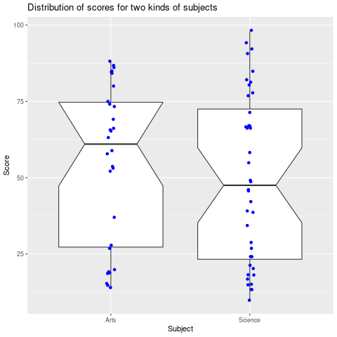
So with your example data: WellFirst, my internetone should always do some visualizing of the data. For your data, parallel boxplots with data values overlaid is so slow nowa good choice:

Parallel boxplots with overlaid data points

Then we do the permutation test, probably becausebased on difference in means of everybody homeofficing for our friend Corona .the two groups.

meandiff_obs <- diff(with(score_data, tapply(Score, Subject, mean))) # Science - Arts

# Permute 9999 times

perm_dist <- replicate(9999, {tags <- score_data$Subject
    scores <- sample(score_data$Score, length(score_data$Score))
    diff(tapply(scores, tags, mean))
} )

perm_dist <- data.frame(meandiff=c(perm_dist))  

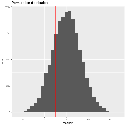
And we can show the results graphically:

Permutation distribution

with the observed meandiff as a red line. Coming back again when it is working

For the record, the code for the plots:

library(ggplot2)
ggplot(score_data, aes(Subject, Score)) +
    geom_boxplot(notch=TRUE) +
    geom_jitter(position=position_jitter(0.03), color="blue") +
    ggtitle("Distribution of scores for two kinds of subjects") 

ggplot(perm_dist, aes(meandiff)) + geom_histogram() +
    geom_vline(xintercept=meandiff_obs, color="red") +
    ggtitle("Permutation distribution")

... and for reading the data:

score_data_text <-
  "   Arts  Science
88  20
85  13
84  58
74  66
66  49
53  46
63  42
15  46
28  39
65  15
27  78
75  66
19  81
37  67
85  21
80  55
69  94
20  18
73  24
87  27
58  67
86  71
66  13
19  29
19  18
15  85
52  80
54  17
14  98
59  91
0   24
0   82
0   67
0   49
0   39
0   34
0   92
0   10
0   15
0   77"  # Added zeros to simplify reading,  to be removed!

score_data <- read.table(textConnection(score_data_text), header=TRUE)
score_data <- as.list(score_data)
score_data$Arts <- with(score_data, Arts[Arts>0])
score_data <- with(score_data, data.frame(Subject=factor(c(rep("Arts", 30), rep("Science", 40))), Score=c(Arts, Science)) )

So with your example data: Well, my internet is so slow now, probably because of everybody homeofficing for our friend Corona ... Coming back again when it is working ...

So with your example data: First, one should always do some visualizing of the data. For your data, parallel boxplots with data values overlaid is a good choice:

Parallel boxplots with overlaid data points

Then we do the permutation test, based on difference in means of the two groups.

meandiff_obs <- diff(with(score_data, tapply(Score, Subject, mean))) # Science - Arts

# Permute 9999 times

perm_dist <- replicate(9999, {tags <- score_data$Subject
    scores <- sample(score_data$Score, length(score_data$Score))
    diff(tapply(scores, tags, mean))
} )

perm_dist <- data.frame(meandiff=c(perm_dist))  

And we can show the results graphically:

Permutation distribution

with the observed meandiff as a red line.

For the record, the code for the plots:

library(ggplot2)
ggplot(score_data, aes(Subject, Score)) +
    geom_boxplot(notch=TRUE) +
    geom_jitter(position=position_jitter(0.03), color="blue") +
    ggtitle("Distribution of scores for two kinds of subjects") 

ggplot(perm_dist, aes(meandiff)) + geom_histogram() +
    geom_vline(xintercept=meandiff_obs, color="red") +
    ggtitle("Permutation distribution")

... and for reading the data:

score_data_text <-
  "   Arts  Science
88  20
85  13
84  58
74  66
66  49
53  46
63  42
15  46
28  39
65  15
27  78
75  66
19  81
37  67
85  21
80  55
69  94
20  18
73  24
87  27
58  67
86  71
66  13
19  29
19  18
15  85
52  80
54  17
14  98
59  91
0   24
0   82
0   67
0   49
0   39
0   34
0   92
0   10
0   15
0   77"  # Added zeros to simplify reading,  to be removed!

score_data <- read.table(textConnection(score_data_text), header=TRUE)
score_data <- as.list(score_data)
score_data$Arts <- with(score_data, Arts[Arts>0])
score_data <- with(score_data, data.frame(Subject=factor(c(rep("Arts", 30), rep("Science", 40))), Score=c(Arts, Science)) )
added 511 characters in body
Source Link
kjetil b halvorsen
  • 82.8k
  • 32
  • 201
  • 663

The independence requirement for the t-test is not really relevant here, as you have only one students's data (If you had data for more students, that would be more of an issue) ... but there is also an assumption of normal distribution and that is also doubtful here. You cannot use a paired test as this is not paired data.

I would here use a permutation test. Under the assumption that the scoring is the same for science and non-science courses, the labels science, non-science is just like they were attached arbitrarily to the courses. So you can simulate the permutation distribution of the difference of the means, say, by permuting the labels, say, $R=9999$ times, and each time compute the differences of the means. Draw the histogram, and over that, draw the observed difference as a line.


If you will post a link to yourAfter questions in comments: Why is the independence assumption not relevant in this case with data from only one person? Because of exchangeability. Under the null hypothesis of no difference between groups, the data is exchangeable, I can show how to dosee for instance Wilcoxon signed rank test independence assumption and search this site.

So with your example data: Well, my internet is so slow now, probably because of everybody homeofficing for our friend Corona ... Coming back again when it is working ...

The independence requirement for the t-test is not really relevant here, as you have only one students's data (If you had data for more students, that would be more of an issue) ... but there is also an assumption of normal distribution and that is also doubtful here. You cannot use a paired test as this is not paired data.

I would here use a permutation test. Under the assumption that the scoring is the same for science and non-science courses, the labels science, non-science is just like they were attached arbitrarily to the courses. So you can simulate the permutation distribution of the difference of the means, say, by permuting the labels, say, $R=9999$ times, and each time compute the differences of the means. Draw the histogram, and over that, draw the observed difference as a line.

If you will post a link to your data, I can show how to do this.

The independence requirement for the t-test is not really relevant here, as you have only one students's data (If you had data for more students, that would be more of an issue) ... but there is also an assumption of normal distribution and that is also doubtful here. You cannot use a paired test as this is not paired data.

I would here use a permutation test. Under the assumption that the scoring is the same for science and non-science courses, the labels science, non-science is just like they were attached arbitrarily to the courses. So you can simulate the permutation distribution of the difference of the means, say, by permuting the labels, say, $R=9999$ times, and each time compute the differences of the means. Draw the histogram, and over that, draw the observed difference as a line.


After questions in comments: Why is the independence assumption not relevant in this case with data from only one person? Because of exchangeability. Under the null hypothesis of no difference between groups, the data is exchangeable, see for instance Wilcoxon signed rank test independence assumption and search this site.

So with your example data: Well, my internet is so slow now, probably because of everybody homeofficing for our friend Corona ... Coming back again when it is working ...

Source Link
kjetil b halvorsen
  • 82.8k
  • 32
  • 201
  • 663
Loading