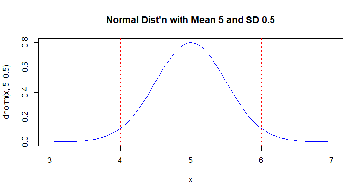
Sampling one individual from a population. In the first situation, The population is distributed normally with mean $\mu = 5$ and standard deviation $\sigma = 0.5.$ Then about 95% of the population lies within the interval $\mu \pm 2\sigma,$ which amounts to the interval $(4, 6).$ Here is a graph of the normal distribution with vertical dotted lines at $4$ and at $6.$ Then 95% of the probability (area) under the curve lies between the dotted lines.
Averaging a large sample from a population. In the second situation, Suppose for the sake of argument that the population has $\mu = 110$ and $\sigma = 20.$ Suppose you take a sample of $n = 100$ people from that distribution and take its sample mean $\bar X.$ Then one can show that $\bar X$ has a normal distribution with mean $\mu_{\bar X} = \mu = 110$ and $\sigma_{\bar X} = \sigma/\sqrt{n} = 20/\sqrt{100} = 20/10 = 2.$
I suppose that sounds very technical. But, intuitively, it makes sense that a sample average must be less variable than the population from which it was drawn. The population has a few people who eat very little pizza and some others who eat pizza moderately and a few who eat massive amounts of pizza. If we sample just one person from the population we could get any of the above types of pizza eaters.
But if we sample a large number of people, we are likely to encounter a broad spectrum of pizza eaters. If we average this diverse sample, we can expect the average to be less variable than the population. This argument doesn't tell you to divide by $\sqrt{n},$ but it does say why the variance of the sample mean is smaller. More on this below.
So $\bar X$ has a 95% chance of being within $2\sigma_{\bar X} = 4$ of $\mu = 110.$ But from data at hand we know $\bar X = 110$ and we're trying to use this sample mean to estimate the unknown population mean. Because be know $\bar X = 110$ and $\mu$ are likely to be 4 units (pizzas) apart, it is reasonable to guess that $\mu$ lies in the interval $\bar X \pm 4.$ We say that a 95% confidence interval for $\mu$ is the interval $110 \pm 4$ or $(106, 114).$
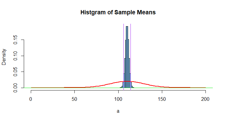
As a simulation experiment, I took many samples of size $n = 100$ from a normal population with mean $\mu = 100$$\mu = 110$ and standard deviation $\sigma = 20.$ I took the average $A = \bar X$ of each of the many samples. (Because simulation is cheap, I took a million samples of size $n = 100.)$
The histogram of all these $A$'a is shown below along with the (much more spread out) density curve of a normal distribution with mean $\mu$ and standard deviation $\sigma = 10.$ The vertical purple lines are at $106$ and $114.$
Notes: (1) According to the scale used to plot the second figure the total area underneath the red curve is $1.$ Also, the total area within the histogram bars is $1.$ Roughly speaking, the histogram is $1/10$th as 'wide' as the curve, so it needs to be $10$ times as 'tall' in order for both areas to be $1.$
(2) In case it is of interest to anyone, the R code for the simulation and the second figure is given below.
a = replicate(10^6, mean(rnorm(100, 110, 20)))
hist(a, prob=T, col="skyblue2", xlim=c(0,200),
     main="Histgram of Sample Means")
 curve(dnorm(x,110,20), add=T, lwd=2, col="red")
 abline(h=0, col="green2")
 abline(v=c(106, 114), col="purple")


