It is decidedly out of the ordinary.

The reason is that counts like these tend will have Poisson distributions. This implies their inherent variance equals the count. For counts near $100,$ that variance of $100$ means the standard deviations are nearly $10.$ Unless there is extreme serial correlation of the results (which is not biologically or medically plausible), this means the majority of individual values ought to deviate randomly from the underlying hypothesized "true" rate by up to $10$ (above and below) and, in an appreciable number of cases (around a third of them all) should deviate by more than that.

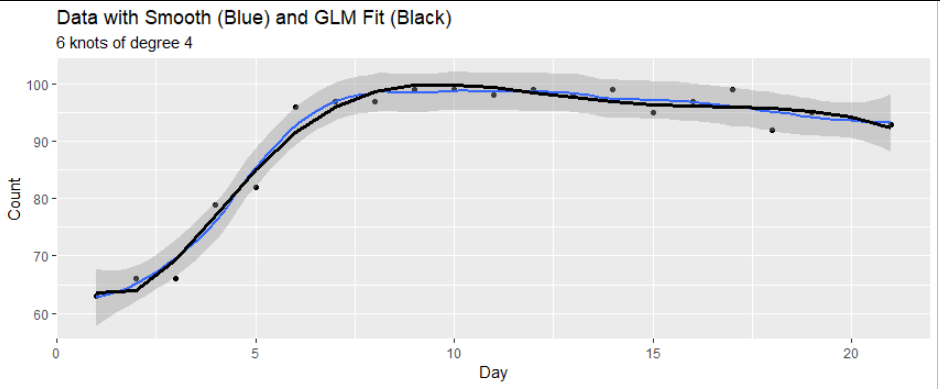
This is difficult to test in a truly robust manner, but one way would be to overfit the data, attempting to describe them very accurately, and see how large the residuals tend to be. Here, for instance, are two such fits, a lowess smooth and an overfit Poisson GLM:

The variance of the residuals for this Generalized Linear Model (GLM) fit (on a logit scale) is only $0.07.$ For other models with (visually) close fits the variance tends to be from $0.05$ to $0.10.$ This is too small.

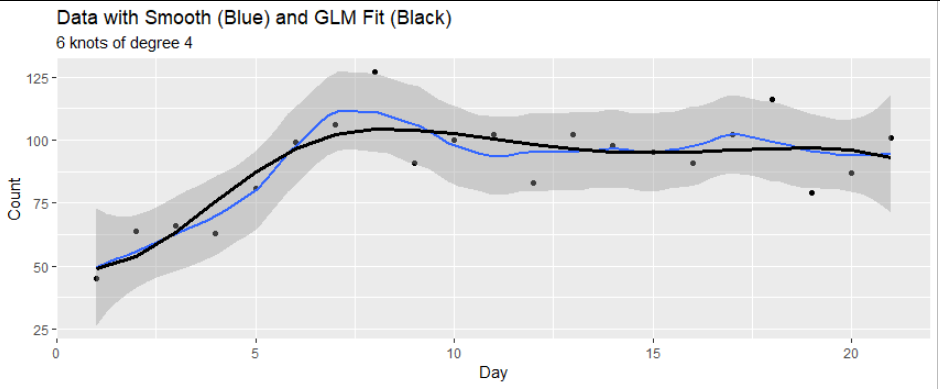
How can you know? Bootstrap it. I chose a parametric bootstrap in which the data are replaced by independent Poisson values drawn from distributions whose parameters equal the predicted values. Here is one such bootstrapped dataset:

You can see how much more the individual values fluctuate than before, and by how much.

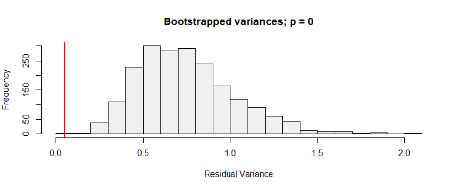
Doing this $5000$ times produced $5001$ variances (in two or three seconds of computation). Here is their histogram:

The vertical red line marks the value of the variance for the data.

(In a well-fit model, the mean of this histogram should be close to $1.$ The mean is $0.75,$ a little less than $1,$ giving an indication of the degree of overfitting.)

The p-value for this test is the fraction of those $5001$ variances that are equal to or less than the observed variance. Since every bootstrapped variance was larger, the p-value is only $1/5001,$ essentially zero.

I repeated this calculation for other models. In the R code below, the models vary according to the number of knots k and degree d of the spline. In every case the p-value remained at $1/5001.$

This confirms the suspicious look of the data. Indeed, if you hadn't stated that these are counts of cases, I would have guessed they were percentages of something. For percentages near $100$ the variation will be very much less than in this Poisson model and the data would not look so suspicious.

This is the code that produced the first and third figures. (A slight variant produced the second, replacing X by X0 at the beginning.)

y <- c(63, 66, 66, 79, 82, 96, 97, 97, 99, 99, 98, 99, 98, 
       99, 95, 97, 99, 92, 95, 94, 93)
X <- data.frame(x=seq_along(y), y=y)

library(splines)
k <- 6
d <- 4
form <- y ~ bs(x, knots=k, degree=d)
fit <- glm(form, data=X, family="poisson")
X$y.hat <- predict(fit, type="response")

library(ggplot2)
ggplot(X, aes(x,y)) + 
  geom_point() + 
  geom_smooth(span=0.4) + 
  geom_line(aes(x, y.hat), size=1.25) + 
  xlab("Day") + ylab("Count") + 
  ggtitle("Data with Smooth (Blue) and GLM Fit (Black)",
          paste(k, "knots of degree", d))

stat <- function(fit) var(residuals(fit))
X0 <- X
set.seed(17)
sim <- replicate(2e3, {
  X0$y <- rpois(nrow(X0), X0$y.hat)
  stat(glm(form, data=X0, family="poisson"))
})

z <- stat(fit)
p <- mean(c(1, sim <= z))
hist(c(z, sim), breaks=25, col="#f0f0f0",
     xlab = "Residual Variance", 
     main=paste("Bootstrapped variances; p =", round(p, log10(length(sim)))))
abline(v = z, col='Red', lwd=2)