TL;DR: 11 (possibly 10).

I got this by simulation, and to be honest, I think a closed formula will be quite painful to derive. Here is my thinking.

First, we can quite easily derive the probability mass function (PMF) $(p_k)$ for the sum of 6d6 by convolution. In R:

n_dice <- 6
probs <- rep(1/6,6)
for ( ii in 2:n_dice ) probs <- convolve(probs,rep(1/6,6),type="open")
names(probs) <- n_dice:(6*n_dice)

Now, it's not overly hard to derive the probability that the first three roll totals $R_1, R_2, R_3$ fulfill your condition, i.e., the probability $q_1$ that your dice rolling stops after 1 step:

$$ \begin{align*} q_1 = \; & P(R_1\geq R_2\geq R_3) \\ = \; & \sum_{k=6}^{36} P(R_1\geq k)P(R_2=k)P(R_3\leq k) \\ = \; & \sum_{k=6}^{36}\bigg(\sum_{j=k}^{36}p_j\bigg)p_k\bigg(\sum_{j=6}^k p_j\bigg) \\ \approx \; & 0.2016245. \end{align*} $$

In R:

q_1 <- sum(sapply(seq_along(probs),function(kk)sum(probs[kk:length(probs)])*probs[kk]*sum(probs[1:kk])))

We can still find the probability $q_2$ that you stop after the second step:

$$ \begin{align*} q_2 = \; & P(R_1< R_2\geq R_3\geq R_4) \\ = \; & \sum_{k=6}^{36} P(R_1<R_2)P(R_2\geq k)P(R_3=k)P(R_4\leq k) \\ = \; & \sum_{k=6}^{36}\bigg(\sum_{j=k}^{36}\Big(\sum_{i=6}^{j-1}p_i\Big)p_j\bigg)p_k\bigg(\sum_{j=6}^k p_j\bigg) \\ \approx \; & 0.1409793. \end{align*} $$

In R again:

q_2 <- 0
for ( kk in 6:length(probs) ) {
    q_2 <- q_2 +
        sum(sapply(kk:length(probs),function(jj)sum(probs[1:(jj-1)])*probs[jj])) *
        probs[kk] *
        sum(probs[1:kk])
}
q_2

Interestingly, the precise same calculation gives us $q_3$, since the condition to stop at step 3 is $R_2<R_3\geq R_4\geq R_5$, and $R_1$ doesn't matter. So since all rolls are iid,

$$ q_3 = P(R_2<R_3\geq R_4\geq R_5) = P(R_1< R_2\geq R_3\geq R_4) = q_2 \approx 0.1409793. $$

Unfortunately, the problem starts about here. To calculate $q_4$, we have to get a handle on why the rolling didn't stop in steps 1-3. We know that $R_3<R_4\geq R_5\geq R_6$ (because we are stopping in step 4), but this relationship imposes a condition on our previous rolls: given this condition, the third roll is more likely to be lower, and since we didn't stop in step 1, this changes the conditional distributions of $R_1$ and $R_2$. The cases get complicated quickly.

So unless you are happy with a stopping probability $<q_1+q_2+q_3\approx 0.483583$ (for which the formulas above give the exact probabilities), the best you can do is likely to simulate. Here is a simulation of the stopping probabilities in R:

n_sims <- 1e6
results <- rep(0,n_sims)
pb <- winProgressBar(max=n_sims)
for ( ii in 1:n_sims ) {
    setWinProgressBar(pb,ii,paste(ii,"of",n_sims))
    set.seed(ii)
    roll_1 <- sum(sample(1:6,n_dice,replace=TRUE))
    roll_2 <- sum(sample(1:6,n_dice,replace=TRUE))
    roll_3 <- sum(sample(1:6,n_dice,replace=TRUE))
    counter <- 1
    while ( roll_1<roll_2 | roll_2<roll_3 ) {
        roll_1 <- roll_2
        roll_2 <- roll_3
        roll_3 <- sum(sample(1:6,n_dice,replace=TRUE))
        counter <- counter+1
    }
    results[ii] <- counter
}
close(pb)
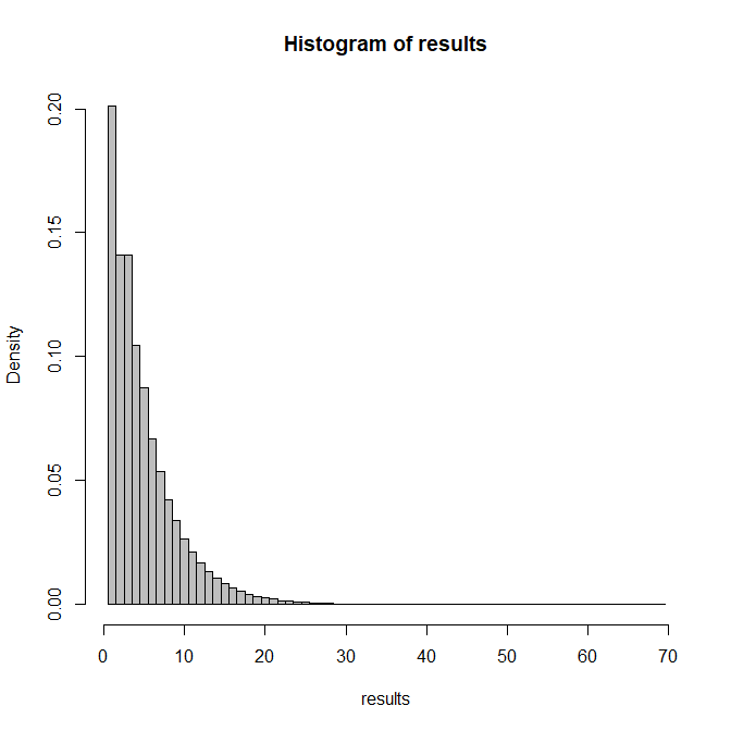
hist(results,breaks=seq(0.5,max(results)+0.5),col="grey",freq=FALSE)

Note how the first three tabulated frequencies are close to the $q_1, q_2, q_3$ we calculated above:

> table(results)/n_sims
results
       1        2        3        4        5        6        7        8        9       10       11       12       13       14       15       16       17       18       19       20       21       22       23       24       25       26 
0.201307 0.140820 0.141095 0.104467 0.087303 0.066984 0.053460 0.042390 0.033982 0.026595 0.021161 0.016777 0.013222 0.010485 0.008337 0.006501 0.005204 0.004071 0.003291 0.002639 0.002096 0.001638 0.001300 0.001002 0.000833 0.000668 
      27       28       29       30       31       32       33       34       35       36       37       38       39       40       41       42       43       44       45       46       47       48       49       50       51       52 
0.000500 0.000372 0.000298 0.000217 0.000204 0.000156 0.000124 0.000110 0.000072 0.000068 0.000047 0.000040 0.000036 0.000027 0.000024 0.000019 0.000009 0.000013 0.000005 0.000005 0.000007 0.000006 0.000002 0.000002 0.000002 0.000001 
      53       54       58       61       66       69 
0.000001 0.000001 0.000001 0.000001 0.000001 0.000001 

Finally, to get the number you are looking for, we look at the cumulative frequencies and note where this exceeds 90%:

> cumsum(table(results)/n_sims)
       1        2        3        4        5        6        7        8        9       10       11       12       13       14       15       16       17       18       19       20       21       22       23       24       25       26 
0.201307 0.342127 0.483222 0.587689 0.674992 0.741976 0.795436 0.837826 0.871808 0.898403 0.919564 0.936341 0.949563 0.960048 0.968385 0.974886 0.980090 0.984161 0.987452 0.990091 0.992187 0.993825 0.995125 0.996127 0.996960 0.997628 
      27       28       29       30       31       32       33       34       35       36       37       38       39       40       41       42       43       44       45       46       47       48       49       50       51       52 
0.998128 0.998500 0.998798 0.999015 0.999219 0.999375 0.999499 0.999609 0.999681 0.999749 0.999796 0.999836 0.999872 0.999899 0.999923 0.999942 0.999951 0.999964 0.999969 0.999974 0.999981 0.999987 0.999989 0.999991 0.999993 0.999994 
      53       54       58       61       66       69 
0.999995 0.999996 0.999997 0.999998 0.999999 1.000000 

So our result is 11 (but because of sampling variability, there is a small chance that it's actually 10).