added 3611 characters in body
Source Link

If you need the subsuming categories, a completely different approach may be taken. Here, it would be useful to know the relations between the categories, which may be 'subsuming' and 'identical' and display or store them in a useful manner. For this purpose, I suggest using a graph.

The code below is a function and a short script that starts after the definition of rmat in the first answer. This time, it's not a cluster analysis but the relations between the categories are assessed and stored in a graph object. This may be plotted and analyzed further:

## This is a function to compute all overlaps and subsuming relations.

overlaps = function(ta,row=T,sub=F){ ## Takes a dichotomous table and computes the overlap
  if(row==F){ta=t(ta)}
  ncas = dim(ta)[1]
  outmat = matrix(0,nrow=ncas,ncol=ncas)
  outmat2 = matrix(0,nrow=ncas,ncol=ncas)
  
  ilist = list()
  slist = list()
  for(n1 in 1:ncas){
    ilist[[n1]]=c(NA)
    slist[[n1]]=c(NA)
    for(n2 in 1:ncas){
      if(n1!=n2){
        d = ta[n1,]-ta[n2,]
        if(min(d)==max(d)){
          outmat[n1,n2]=1 ## Equality
          ilist[[n1]]=c(ilist[[n1]],n2)
        }else if(min(d)==0 & max(ta[n2,]>0)){
          outmat[n1,n2]=2 ## Subsuming
          slist[[n1]]=c(slist[[n1]],n2)
        }
      }
      
    }
  }
  rownames(outmat)=colnames(outmat)=rownames(ta)
  
  if(!sub){
    for(i in 1:length(slist)){
      so = c()
      for(s in slist[[i]]){
        so = c(so,slist[[s]])
      }
      for(s in slist[[i]]){
        if(s %in% so){
          outmat[i,s]=0
        }
      }
    }
  }
  return(outmat)
}

###################################################
### Here follows the short script:

library(igraph)
adjmat = overlaps(rmat,sub=F) ## Create an adjacency matrix with the option that subsuming edges are removed

g = graph_from_adjacency_matrix(adjmat, mode="directed",weighted=T) ## Create a graph
g = delete.edges(g,E(g)[E(g)$weight==0]) ## Remove all edges with weight zero (no link)

## Graph cosmetics
E(g)$arrow.size=.5
E(g)$width = 1
E(g)$color = "#30a030"
E(g)$color[E(g)$weight==2] = "#f08080"
V(g)$color = c("#eeeeff")
V(g)$frame.color=NA
V(g)$label.family="Arial"
V(g)$label.cex=.8
V(g)$shape="circle"
V(g)$size=20

chief = rownames(adjmat)[degree(g,mode="in")==0] ## Make the nodes which are not subsumed the root of the tree
l = layout_as_tree(g,root=chief) ## Construct the tree
plot(g,layout=l) ## Plot the tree

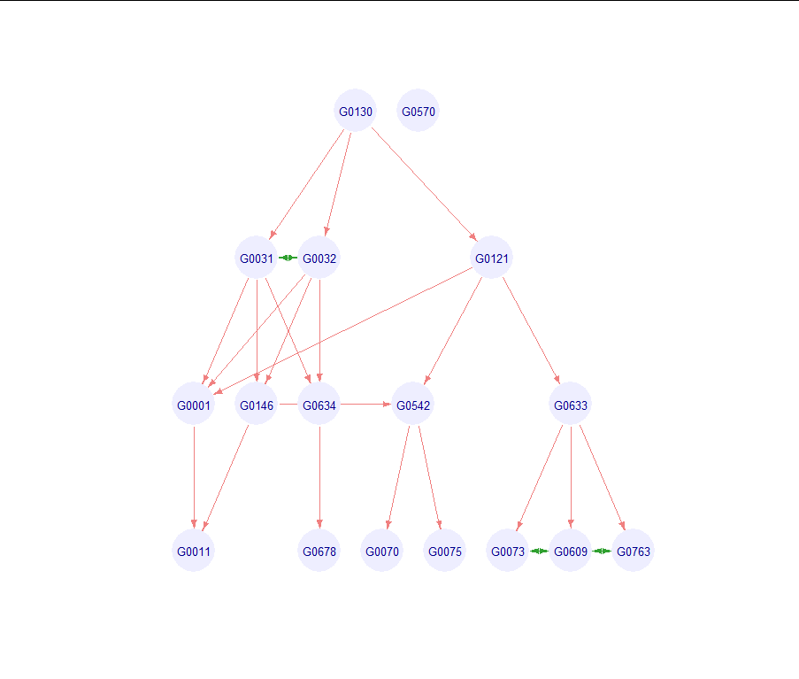
The result of this script (again, only for the first 100 elements of your data) would be the following tree representation where red arrows mean 'subsuming' and green arrows mean 'is identical'. So, you see that there is one unique category in these first 100, which is 570. All others are subsumed by 130. Categories 31 and 32, as well as 73, 609, and 763 are identical.

As you can see, this already begins to get complicated. It gets even worse if you try to plot all the data in this way. But the nice thing about graphs is that you can analyze pieces of them and look at detail graphs (elements that are identical, elements with many subsuming elements...). Probably your categories even make sense to you, which would make the exploration easier.

enter image description here

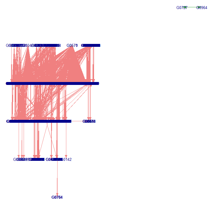
This would be the complete graph. From this, you can only gather that 727 and 964 are identical and don't have any connection to the others. Everything else is a blur.

enter image description here

If you need the subsuming categories, a completely different approach may be taken. Here, it would be useful to know the relations between the categories, which may be 'subsuming' and 'identical' and display or store them in a useful manner. For this purpose, I suggest using a graph.

The code below is a function and a short script that starts after the definition of rmat in the first answer. This time, it's not a cluster analysis but the relations between the categories are assessed and stored in a graph object. This may be plotted and analyzed further:

## This is a function to compute all overlaps and subsuming relations.

overlaps = function(ta,row=T,sub=F){ ## Takes a dichotomous table and computes the overlap
  if(row==F){ta=t(ta)}
  ncas = dim(ta)[1]
  outmat = matrix(0,nrow=ncas,ncol=ncas)
  outmat2 = matrix(0,nrow=ncas,ncol=ncas)
  
  ilist = list()
  slist = list()
  for(n1 in 1:ncas){
    ilist[[n1]]=c(NA)
    slist[[n1]]=c(NA)
    for(n2 in 1:ncas){
      if(n1!=n2){
        d = ta[n1,]-ta[n2,]
        if(min(d)==max(d)){
          outmat[n1,n2]=1 ## Equality
          ilist[[n1]]=c(ilist[[n1]],n2)
        }else if(min(d)==0 & max(ta[n2,]>0)){
          outmat[n1,n2]=2 ## Subsuming
          slist[[n1]]=c(slist[[n1]],n2)
        }
      }
      
    }
  }
  rownames(outmat)=colnames(outmat)=rownames(ta)
  
  if(!sub){
    for(i in 1:length(slist)){
      so = c()
      for(s in slist[[i]]){
        so = c(so,slist[[s]])
      }
      for(s in slist[[i]]){
        if(s %in% so){
          outmat[i,s]=0
        }
      }
    }
  }
  return(outmat)
}

###################################################
### Here follows the short script:

library(igraph)
adjmat = overlaps(rmat,sub=F) ## Create an adjacency matrix with the option that subsuming edges are removed

g = graph_from_adjacency_matrix(adjmat, mode="directed",weighted=T) ## Create a graph
g = delete.edges(g,E(g)[E(g)$weight==0]) ## Remove all edges with weight zero (no link)

## Graph cosmetics
E(g)$arrow.size=.5
E(g)$width = 1
E(g)$color = "#30a030"
E(g)$color[E(g)$weight==2] = "#f08080"
V(g)$color = c("#eeeeff")
V(g)$frame.color=NA
V(g)$label.family="Arial"
V(g)$label.cex=.8
V(g)$shape="circle"
V(g)$size=20

chief = rownames(adjmat)[degree(g,mode="in")==0] ## Make the nodes which are not subsumed the root of the tree
l = layout_as_tree(g,root=chief) ## Construct the tree
plot(g,layout=l) ## Plot the tree

The result of this script (again, only for the first 100 elements of your data) would be the following tree representation where red arrows mean 'subsuming' and green arrows mean 'is identical'. So, you see that there is one unique category in these first 100, which is 570. All others are subsumed by 130. Categories 31 and 32, as well as 73, 609, and 763 are identical.

As you can see, this already begins to get complicated. It gets even worse if you try to plot all the data in this way. But the nice thing about graphs is that you can analyze pieces of them and look at detail graphs (elements that are identical, elements with many subsuming elements...). Probably your categories even make sense to you, which would make the exploration easier.

enter image description here

This would be the complete graph. From this, you can only gather that 727 and 964 are identical and don't have any connection to the others. Everything else is a blur.
enter image description here

Source Link

You could use a hierachical cluster analysis to determine the categories that resemble each other most.

I used your data do create the following script that will notify you about the most proximal elements. Note, that I only take the first 100 cases for this example. But it works well with the complete dataset and takes below 1 minute.

## Read your data as a 2-column dataset
d = read.table("relations.txt",header=T,sep=",",stringsAsFactors = F)

d=d[1:100,]

## Create a matrix with all relations
rmat = as.matrix(table(d$category,d$item_code))
dim(rmat)

## Compute a distance matrix and do a hierarchical cluster analysis
dm = dist(rmat)
cl = hclust(dm)


## Set a threshold for distance (as it es "euclidian", the distance is the square root of disagreements)
threshold = 2  ## Less than 4 diverging links

## Get the number of clusters if you cut at this threshold and cut the tree
nclus = length(cl$height)-length(cl$height[cl$height>threshold])
t =cutree(cl,k=nclus)

## Extract all clusters below the threshold
sizes = table(t)
items = t[t %in% names(sizes[sizes>1])]

## Order the items
items = items[order(items)]

## Print the result:
for(c in unique(items)){
  print(paste(names(items[items==c]),collapse="; "))
}

## Plot the tree (only useful if it is small)
plot(cl)

The output of this script for the first 100 cases would be:

[1] "G0031; G0032; G0130"
[1] "G0070; G0542"
[1] "G0073; G0609; G0763"

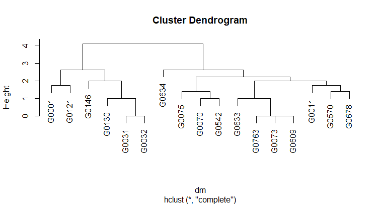
From this, you can see that the categories 31,32, and 130 are very similar to each other. Just like 70 and 542 or 73,609, and 763. This is also visible in the dendrogram below.

Dendrogram