added marginal effects plot since the OP doesn't understand how contrast coding works
Source Link
conjugateprior
  • 21.3k
  • 2
  • 63
  • 90

How about this. Let's make up some data where there really is a day effect

## dates of each day of 2012
days2012 <- seq(as.Date("2012-01-01"), as.Date("2012-12-31"), by="day")

## make variables representing interesting temporal units
dta <- data.frame(date=days2012, day=weekdays(days2012), month=months(days2012))

## specify average rates that are higher on Wednesdays
dta$muY <- ifelse(dta$day=='Wednesday', 10, 5)

## generate random count data from average rates  
dta$Y <- rpois(rep(1, nrow(dta)), dta$muY)

To spot the fact that Wednesdays are special in this data set you can use a generalised linear model. This one asks whether rates vary by month or day or both:

mod <- glm(Y ~ day + month, data=dta, family=poisson)
summary(mod)

which gives a nice big effect for the dummy variable that represents Wednesday.

To avoid the dummy variable contrasts obscuring the interpretation you can look at the marginal effects

library(effects) 
plot(effect("day", mod))

which again gives a big spike for Wednesday while operating on the scale of the observed counts.
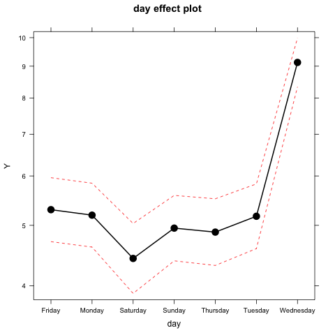
enter image description here

How about this. Let's make up some data where there really is a day effect

## dates of each day of 2012
days2012 <- seq(as.Date("2012-01-01"), as.Date("2012-12-31"), by="day")

## make variables representing interesting temporal units
dta <- data.frame(date=days2012, day=weekdays(days2012), month=months(days2012))

## specify average rates that are higher on Wednesdays
dta$muY <- ifelse(dta$day=='Wednesday', 10, 5)

## generate random count data from average rates  
dta$Y <- rpois(rep(1, nrow(dta)), dta$muY)

To spot the fact that Wednesdays are special in this data set you can use a generalised linear model. This one asks whether rates vary by month or day or both:

mod <- glm(Y ~ day + month, data=dta, family=poisson)
summary(mod)

which gives a nice big effect for the dummy variable that represents Wednesday.

To avoid the dummy variable contrasts obscuring the interpretation you can look at the marginal effects

library(effects) 
plot(effect("day", mod))

which again gives a big spike for Wednesday while operating on the scale of the observed counts.

enter image description here

Source Link
conjugateprior
  • 21.3k
  • 2
  • 63
  • 90

How about this. Let's make up some data where there really is a day effect

## dates of each day of 2012
days2012 <- seq(as.Date("2012-01-01"), as.Date("2012-12-31"), by="day")

## make variables representing interesting temporal units
dta <- data.frame(date=days2012, day=weekdays(days2012), month=months(days2012))

## specify average rates that are higher on Wednesdays
dta$muY <- ifelse(dta$day=='Wednesday', 10, 5)

## generate random count data from average rates  
dta$Y <- rpois(rep(1, nrow(dta)), dta$muY)

To spot the fact that Wednesdays are special in this data set you can use a generalised linear model. This one asks whether rates vary by month or day or both:

mod <- glm(Y ~ day + month, data=dta, family=poisson)
summary(mod)

which gives a nice big effect for the dummy variable that represents Wednesday.