By adapting the (simple, recursive) method for approximating QQ plots I described at https://stats.stackexchange.com/a/35268/919, you can efficiently find a precise (piecewise linear) approximation of the full empirical quantile function using just a few values, typically a few hundred to a few thousand even for a batch of a billion numbers (depending on how precise the summary needs to be). It is fast and straightforward to combine two such summaries to produce the full empirical quantile function of the combined datasets.

This algorithm requires $O(n\log(n))$ computational effort to process a batch of $n$ numbers and, because it is a divide-and-conquer algorithm, it is highly parallelizable. This makes it practicable even for large datasets; for instance, on a single core R requires only about four minutes to process a dataset of one billion ($10^9$) numbers.

The crux of the matter is to compute the quantile function $F^{-1}$ of a mixture of two distributions $F_X$ and $F_Y$ in terms of those distributions and their quantile functions $F_X^{-1}$ and $F_Y^{-1}.$ Let $p_X$ and $p_Y,$ with $p_X+p_Y=1,$ be the (positive) mixture weights. This means that for any number $x,$

$$F(x) = p_X F_X(x) + p_Y F_Y(x).\tag{*}$$

Let $0 \lt q \lt 1$ (the question concerns the median, where $q=1/2$) and suppose we want to find the quantile $F^{-1}(q).$ By definition, this is the smallest $x$ among the numbers for which $F(x) \ge q.$ Replacing $F$ by the foregoing expression and algebraically rearranging gives

$$F_X(x) \ge \frac{1}{p_X}\left(q - p_Y F_Y(x)\right),$$

which means

$$x = F_X^{-1}\left(\frac{1}{p_X}\left(q - p_Y F_Y(x)\right)\right).$$

A simple search for the smallest zero of

$$g(x) = F_X^{-1}\left(\frac{1}{p_X}\left(q - p_Y F_Y(x)\right)\right)-x\tag{**}$$

thereby computes the $q$ quantile of $F.$

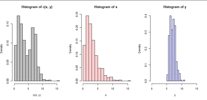
As an example, here are two small datasets of 700 and 300 numbers each, named x and y.

The challenge is to approximate the median (or any other quantile) of the left (combined) distribution based on small summaries of its component distributions (shown in color). For these data, the proposed algorithm summarizes x using $34$ (value, quantile) pairs and it summarizes y using just $10$ (value, quantile) pairs. These summaries approximate the quantile functions to within a maximum error of $0.5\%$ of the range of all the data. (The amount of allowable error can be set to anything, even zero. Zero is an effective choice for discrete data: in this case, the algorithm is equivalent to tabulating the values in each dataset.)

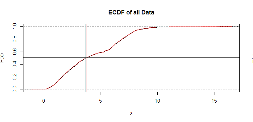
Here is a plot of the empirical distribution function of all the data, $F$ (black), on which is superimposed the mixture distribution $(*)$ as computed from the approximate ECDFs for $F_X$ and $F_Y$ (shown in red):

There are two vertical lines shown: a gray one is located at the true median of the combined data while the red one is located at the root of $g$ (equation $(**)$) computed using the approximate ECDFs. Indeed, they differ by only $0.03,$ which is less than $0.5\%$ of the full range of the data, as intended.

This is the R code that generated the examples. It implements a quantile/distribution function approximator, quantilefun, and shows how to use it for computing quantiles of mixtures of two distributions. It uses the built-in, robust uniroot function to find the mixture quantiles. Because the approximating functions are piecewise linear, they are fast to evaluate, making the search for roots reasonably efficient.

#
# Compute an approximation to the empirical quantile function.
# It will be accurate everywhere to within the given relative tolerance
# (a multiple of the range of `x`).
#
quantilefun <- function(x, tol=0.005) {
  x <- sort(x[!is.na(x)])
  n <- length(x)
  if (n <= 1) stop("need at least two non-NA values to interpolate.")
  threshold <- tol * diff(range(x))
  #
  # Find an index i <= k <= j at which x[k] departs most from the linear
  # interpolator of x[i] and x[j].  Assumes i <= j.
  # Returns a list of the index and the discrepancy.
  #
  f <- function(i,j) {
    beta <- (x[j] - x[i]) / (j - i) 
    dy <- abs(x[i:j] - x[i] - beta * (i:j - i))
    k <- which.max(abs(dy))
    list(k=k+i-1, dy=dy[k])
  }
  #
  # Locate the key indexes into `x` between `i` and `j`.
  # Returns them in ascending order.
  #
  keys <- function(i, j) {
    k <- f(i, j)
    if (abs(k$dy) <= threshold) return(integer())
    c(keys(i,k$k), k$k, keys(k$k,j))
  }
  k <- c(1, keys(1, n), n)
  q <- (k-1)/(n-1)
  #
  # Although only `Indexes` and `Values` are needed, additional summaries
  # are returned for ease of use.
  #
  list(Indexes=k, 
       Values=x[k],
       Range=x[c(1,n)],
       Tolerance=tol,
       Threshold=threshold,
       Quantile=approxfun(q, x[k], yleft=x[1], yright=x[n]), 
       F=approxfun(x[k], q, yleft=0, yright=1))
}
#------------------------------------------------------------------------------#
#
# Create test data.
# It is most difficult to combine datasets with very different quantiles.
#
set.seed(17)
x <- rgamma(7e2, 2, 2/3)
y <- rgamma(3e2, 4, 2) + 5
#
# Compute the approximate empirical distribution functions.
#
tol <- 5e-3
r.x <- range(x)
r.y <- range(y)
n.x <- length(x)
n.y <- length(y)
r <- range(c(r.x, r.y))
n <- n.x + n.y
system.time({
  f.x <- quantilefun(x, tol * diff(r) / diff(r.x))
  f.y <- quantilefun(y, tol * diff(r) / diff(r.y))
})
#
# Estimate the median of the combined data using only the approximate ECDFs.
#
system.time({
  f <- function(x, q=1/2) f.x$Quantile(n/n.x * (q - n.y/n * f.y$F(x))) - x
  median.combined <- uniroot(f, r, tol=1e-12)$root
})
#
# Display the median and the estimated median.
#
median <- median(c(x, y))
d <- -floor(log10(f.x$Threshold))
(c(Median=round(median,d),
   `Combined estimate`=round(median.combined, d),
   Threshold=round(f.x$Threshold, d)))
(c(N = length(f.x$Indexes) + length(f.y$Indexes)))
#
# Plot the combined ECDF.
#
if (n < 1e5) {
  plot(ecdf(c(x,y)), main="ECDF of all Data", ylab=expression(F(x)))
  #
  # Superimpose the combined approximations.
  #
  curve((n.x * f.x$F(x) + n.y * f.y$F(x)) / n, add=TRUE, col="#f0000080", lwd=2)
  #
  # Plot the median and its estimate.
  #
  abline(v = c(median, median.combined), col=c("Gray", "Red"), lwd=2)
  abline(h = 1/2, lwd=2)
}
#
# Plot the histograms.
#
par(mfrow=c(1,3))
hist(c(x,y), freq=FALSE, col="Gray")
hist(x, xlim=range(c(x,y)), freq=FALSE, col="#ffd0d0")
hist(y, xlim=range(c(x,y)), freq=FALSE, col="#d0d0ff")
par(mfrow=c(1,1))