added coverage
Source Link
R. Cox
  • 179
  • 8

Coverage

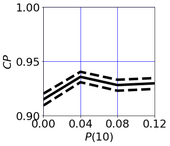
I think the coverage is around 93%, slightly under the target 95%.

enter image description here

Figure 3, Coverage Probability (CP) against P(10)

I assessed it with a simulation.

Coverage changes with probability, so it would be good to try it with various values of the probabilities of the four possible outcomes (P11, P10, P01, P00). Unfortunately, running many values of each P would take too long. Instead, I used MultinomCI to get the Wilson interval for each P. This gave:

      Est   Low     High
P(11) 0.393 0.236   0.576
P(10) 0.000 0.000   0.121
P(01) 0.214 0.102   0.395
P(00) 0.393 0.236   0.576

I gave the name Prob to the vector [P11, P10, P01, P00]

sum (Prob) = 1

I took the range of likely values for P10 and assumed that as P10 increases, P01 decreases equally.

I assessed 4 values of Prob:

Prob = [0.3, 0.0,  0.3,  0.4]
Prob = [0.3, 0.04, 0.26, 0.4]
Prob = [0.3, 0.08, 0.22, 0.4]
Prob = [0.3, 0.12, 0.18, 0.4]

I ran it with:

n       =  28
runs    =  1000
reps    =  10000

which took 41.5 hours.

Last, I estimated the 95% CI for the coverage of the 95% CI, again using the Wilson interval.

In Python:

import numpy  as np
import pandas as pd
import time
import rpy2.robjects as ro
import statsmodels.api
import matplotlib.pyplot as plt

start = time.time()

from rpy2.robjects.packages import importr

package_name = "DescTools"

try:
    pkg = importr(package_name)
except:
    ro.r(f'install.packages("{package_name}")')
    pkg = importr(package_name)
pkg

r_string = """CI = MultinomCI(c(11,0,6,11), conf.level=0.95, method="wilson")
"""
ro.r(r_string)
A_C = np.array(ro.r['CI'])

print(' ')
print('Estimate, CI')
print(A_C)
print(' ')

# Control Parameters
n = 28
print('n       = ',n)

nrep = 10 #10000
print('reps    = ',nrep)

runs = 10 #1000
print('runs    = ',runs)
    
P_10s = [0.00, 0.04, 0.08, 0.12]

d_CP = {}
d_Re = {}

for P_10 in P_10s:
    pvals = [.3, P_10, (.3-P_10), .4]
    print('Prob ',pvals)
    print('total P = ',sum(pvals))

    P_11 = pvals[0]
    P_10 = pvals[1]
    P_01 = pvals[2]
    P_00 = pvals[3]

    I_T = (P_11+P_01)/(P_11+P_10)-1
    print('True I  = ',I_T)

    print('Estimate the Coverage Probability using simulation')
    CP = []

    for it in range(nrep):
        
        # Generate the sample data
        li = np.random.multinomial(n, pvals)
        data = pd.DataFrame({'A':[1]*li[0] +[1]*li[1] +[0]*li[2] +[0]*li[3],
                             'B':[1]*li[0] +[0]*li[1] +[1]*li[2] +[0]*li[3]})
    
        # Results
        Lower = {}
        Media = {}
        Upper = {}
        
        # Results
        I_R = []
    
        for R in range(runs):
                
            # Bootstrap size = n
            BooP = data.sample(n, replace=True)
            
            # Data
            X_11 = len(BooP[((BooP.A==1)&(BooP.B==1))])
            X_10 = len(BooP[((BooP.A==1)&(BooP.B==0))])
            X_01 = len(BooP[((BooP.A==0)&(BooP.B==1))])
            X_00 = len(BooP[((BooP.A==0)&(BooP.B==0))])
        
            # Improvement (I) = pB/pA-1
            if X_11+X_10 == 0:
                I_x = 10101 # approx infinity!
            else:
                I_x = (X_11+X_01)/(X_11+X_10)-1
            
            # Results
            I_R.append(I_x)
            
            # CI
            Lower[R] = np.percentile(I_R,  2.5)
            Media[R] = np.percentile(I_R, 50  )
            Upper[R] = np.percentile(I_R, 97.5)
        
        Low = Lower[max(list(Lower.keys()))]
        Med = Media[max(list(Lower.keys()))]
        Hig = Upper[max(list(Lower.keys()))]
    
        # Check whether the interval contains the true value
        if (I_T < Hig) and (I_T > Low):
            CP.append(1)
        else:
            CP.append(0)
    
    end = time.time()
    print('time    = ',end - start)
    print('CP      = ',sum(CP)/len(CP))
    
    # results
    d_Re[P_10] = CP
    d_CP[P_10] = sum(CP)/len(CP)

# CI
CI_Low  = []
CI_High = []
for P_10 in d_CP.keys():
    low, high = statsmodels.stats.proportion.proportion_confint(d_CP[float(P_10)]*nrep,
                                                                nrep,
                                                                alpha=1-0.95,
                                                                method='wilson')
    CI_Low.append(low)
    CI_High.append(high)


print('Plot')
df_G1 = pd.DataFrame({'P_10' : list(d_CP.keys()),
                      'CP'   : list(d_CP.values()),
                      'Lo'   : CI_Low,
                      'Hi'   : CI_High})

fig, ax1 = plt.subplots(1,1)

df_G1.plot(x='P_10', y='Hi', legend=False, ax=ax1, label='95% CI',  linewidth=5, color='k', linestyle='--')
df_G1.plot(x='P_10', y='CP', legend=False, ax=ax1, label='CP',      linewidth=5, color='k', linestyle='-')
df_G1.plot(x='P_10', y='Lo', legend=False, ax=ax1, label='95% CI',  linewidth=5, color='k', linestyle='--')

for item in ([ax1.title, ax1.xaxis.label, ax1.yaxis.label] +
             ax1.get_xticklabels() + ax1.get_yticklabels()):
    item.set_fontsize(22)

plt.xlabel('$P(10)$')
plt.ylabel('$CP$')

plt.xlim([0,0.12])
plt.ylim([0.9,1])

ax1.set_yticks([.9,.95,1])
plt.xticks([0.00, 0.04, 0.08, 0.12])

plt.grid(which='both', color='b')

fig = plt.gcf()
fig.set_size_inches(4,4)
plt.show()
plt.clf()
cut out some non-statistical code
Source Link
R. Cox
  • 179
  • 8
import numpy  as np
import pandas as pd
import pickle
import matplotlib.pyplot as plt

print('Generate the sample data')
data = pd.DataFrame({'A':[1]*11+[0]*6+[0]*11,
                     'B':[1]*11+[1]*6+[0]*11})
print('sample size: ',len(data))
print('')
print('A B X')
print('1 1',len(data[((data.A==1)&(data.B==1))]))
print('1 0',len(data[((data.A==1)&(data.B==0))]))
print('0 1',len(data[((data.A==0)&(data.B==1))]))
print('0 0',len(data[((data.A==0)&(data.B==0))]))
print('')

# Results
I     = {}
Lower = {}
Media = {}
Upper = {}

# Control Parameters
Runs = range(100)
#bootstrap_size = range(len(data))
BS_Max = 100
bootstrap_size = range(BS_Max)

for BS in bootstrap_size:
    #print('bootstrap size ', BS)
    
    # Results
    I_T = {}
    
    for R in Runs:
        
        # Bootstrap
        BooP = data.sample(BS, replace=True)
        
        # Data
        X_11 = len(BooP[((BooP.A==1)&(BooP.B==1))])
        X_10 = len(BooP[((BooP.A==1)&(BooP.B==0))])
        X_01 = len(BooP[((BooP.A==0)&(BooP.B==1))])
        X_00 = len(BooP[((BooP.A==0)&(BooP.B==0))])
        
        # Improvement (I) = pB/pA-1
        if X_11+X_10 == 0:
            I_x = 10101 # approx infinity!
        else:
            I_x = (X_11+X_01)/(X_11+X_10)-1
        
        # Results
        I_T[R] = I_x
    
    # Results
    I[BS] = I_T
    
    # CI
    Lower[BS] = np.percentile(list(I[BS].values()),  2.5)
    Media[BS] = np.percentile(list(I[BS].values()), 50  )
    Upper[BS] = np.percentile(list(I[BS].values()), 97.5)

print('Save')
output = open('MAE_B3_I.py.pkl', 'wb')
pickle.dump(I, output)
output.close()

output = open('MAE_B3_Lower.py.pkl', 'wb')
pickle.dump(Lower, output)
output.close()

output = open('MAE_B3_Media.py.pkl', 'wb')
pickle.dump(Media, output)
output.close()

output = open('MAE_B3_Upper.py.pkl', 'wb')
pickle.dump(Upper, output)
output.close()

print('Plot')
df_G1 = pd.DataFrame({'BS' : bootstrap_size,
                      'I'  : list(Media.values()),
                      'Lo' : list(Lower.values()),
                      'Hi' : list(Upper.values())})

fig, ax1 = plt.subplots(1,1)

df_G1.plot(x='BS', y='Hi', legend=False, ax=ax1, label='95% CI', linewidth=5, color='k', linestyle='--')
df_G1.plot(x='BS', y='I',  legend=False, ax=ax1, label='I',      linewidth=5, color='k', linestyle='-')
df_G1.plot(x='BS', y='Lo', legend=False, ax=ax1, label='95% CI', linewidth=5, color='k', linestyle='--')

for item in ([ax1.title, ax1.xaxis.label, ax1.yaxis.label] +
             ax1.get_xticklabels() + ax1.get_yticklabels()):
    item.set_fontsize(22)

legend = ax1.legend(loc=0, ncol=1, bbox_to_anchor=(0.9, -.3, 1, 1),
           fancybox=True, shadow=False,
           framealpha=1, fontsize=22) # , title='Percentile'
plt.setp(legend.get_title(),fontsize=22)

plt.xlabel('$BS$')
plt.ylabel('$I$')
plt.grid(b=True, which='major', color='b')
plt.grid(b=True, which='minor', color='b')
plt.xlim([0,BS_Max])
plt.ylim([0,2])

fig = plt.gcf()
fig.set_size_inches(4,4)
plt.show()
plt.clf()
print('Generate the sample data')
data = pd.DataFrame({'A':[1]*11+[0]*6+[0]*11,
                     'B':[1]*11+[1]*6+[0]*11})
print('sample size: ',len(data))
print('')
print('A B X')
print('1 1',len(data[((data.A==1)&(data.B==1))]))
print('1 0',len(data[((data.A==1)&(data.B==0))]))
print('0 1',len(data[((data.A==0)&(data.B==1))]))
print('0 0',len(data[((data.A==0)&(data.B==0))]))
print('')

# Results
I     = {}
Lower = {}
Media = {}
Upper = {}

# Control Parameters
Runs = range(100)
#bootstrap_size = range(len(data))
BS_Max = 100
bootstrap_size = range(BS_Max)

for BS in bootstrap_size:
    #print('bootstrap size ', BS)
    
    # Results
    I_T = {}
    
    for R in Runs:
        
        # Bootstrap
        BooP = data.sample(BS, replace=True)
        
        # Data
        X_11 = len(BooP[((BooP.A==1)&(BooP.B==1))])
        X_10 = len(BooP[((BooP.A==1)&(BooP.B==0))])
        X_01 = len(BooP[((BooP.A==0)&(BooP.B==1))])
        X_00 = len(BooP[((BooP.A==0)&(BooP.B==0))])
        
        # Improvement (I) = pB/pA-1
        if X_11+X_10 == 0:
            I_x = 10101 # approx infinity!
        else:
            I_x = (X_11+X_01)/(X_11+X_10)-1
        
        # Results
        I_T[R] = I_x
    
    # Results
    I[BS] = I_T
    
    # CI
    Lower[BS] = np.percentile(list(I[BS].values()),  2.5)
    Media[BS] = np.percentile(list(I[BS].values()), 50  )
    Upper[BS] = np.percentile(list(I[BS].values()), 97.5)
Source Link
R. Cox
  • 179
  • 8

Bootstrap

I tried a bootstrap. It often threw the error:

division by zero

I got around that by assuming:

infinity = approximately 10101

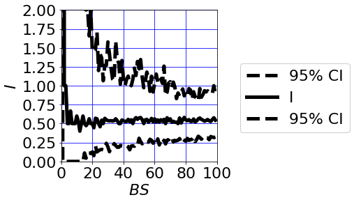
with the resulting estimates:

enter image description here

Figure 1, Improvement (I) against Bootstrap Size (BS) for runs = 100

enter image description here

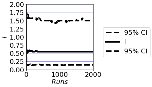
Figure 2, Improvement (I) against against Runs for BS=28

This gave an improvement after 1000 runs with BS=28 of:

55% [14%, 150%]

In Python:

import numpy  as np
import pandas as pd
import pickle
import matplotlib.pyplot as plt

print('Generate the sample data')
data = pd.DataFrame({'A':[1]*11+[0]*6+[0]*11,
                     'B':[1]*11+[1]*6+[0]*11})
print('sample size: ',len(data))
print('')
print('A B X')
print('1 1',len(data[((data.A==1)&(data.B==1))]))
print('1 0',len(data[((data.A==1)&(data.B==0))]))
print('0 1',len(data[((data.A==0)&(data.B==1))]))
print('0 0',len(data[((data.A==0)&(data.B==0))]))
print('')

# Results
I     = {}
Lower = {}
Media = {}
Upper = {}

# Control Parameters
Runs = range(100)
#bootstrap_size = range(len(data))
BS_Max = 100
bootstrap_size = range(BS_Max)

for BS in bootstrap_size:
    #print('bootstrap size ', BS)
    
    # Results
    I_T = {}
    
    for R in Runs:
        
        # Bootstrap
        BooP = data.sample(BS, replace=True)
        
        # Data
        X_11 = len(BooP[((BooP.A==1)&(BooP.B==1))])
        X_10 = len(BooP[((BooP.A==1)&(BooP.B==0))])
        X_01 = len(BooP[((BooP.A==0)&(BooP.B==1))])
        X_00 = len(BooP[((BooP.A==0)&(BooP.B==0))])
        
        # Improvement (I) = pB/pA-1
        if X_11+X_10 == 0:
            I_x = 10101 # approx infinity!
        else:
            I_x = (X_11+X_01)/(X_11+X_10)-1
        
        # Results
        I_T[R] = I_x
    
    # Results
    I[BS] = I_T
    
    # CI
    Lower[BS] = np.percentile(list(I[BS].values()),  2.5)
    Media[BS] = np.percentile(list(I[BS].values()), 50  )
    Upper[BS] = np.percentile(list(I[BS].values()), 97.5)

print('Save')
output = open('MAE_B3_I.py.pkl', 'wb')
pickle.dump(I, output)
output.close()

output = open('MAE_B3_Lower.py.pkl', 'wb')
pickle.dump(Lower, output)
output.close()

output = open('MAE_B3_Media.py.pkl', 'wb')
pickle.dump(Media, output)
output.close()

output = open('MAE_B3_Upper.py.pkl', 'wb')
pickle.dump(Upper, output)
output.close()

print('Plot')
df_G1 = pd.DataFrame({'BS' : bootstrap_size,
                      'I'  : list(Media.values()),
                      'Lo' : list(Lower.values()),
                      'Hi' : list(Upper.values())})

fig, ax1 = plt.subplots(1,1)

df_G1.plot(x='BS', y='Hi', legend=False, ax=ax1, label='95% CI', linewidth=5, color='k', linestyle='--')
df_G1.plot(x='BS', y='I',  legend=False, ax=ax1, label='I',      linewidth=5, color='k', linestyle='-')
df_G1.plot(x='BS', y='Lo', legend=False, ax=ax1, label='95% CI', linewidth=5, color='k', linestyle='--')

for item in ([ax1.title, ax1.xaxis.label, ax1.yaxis.label] +
             ax1.get_xticklabels() + ax1.get_yticklabels()):
    item.set_fontsize(22)

legend = ax1.legend(loc=0, ncol=1, bbox_to_anchor=(0.9, -.3, 1, 1),
           fancybox=True, shadow=False,
           framealpha=1, fontsize=22) # , title='Percentile'
plt.setp(legend.get_title(),fontsize=22)

plt.xlabel('$BS$')
plt.ylabel('$I$')
plt.grid(b=True, which='major', color='b')
plt.grid(b=True, which='minor', color='b')
plt.xlim([0,BS_Max])
plt.ylim([0,2])

fig = plt.gcf()
fig.set_size_inches(4,4)
plt.show()
plt.clf()