Return to Answer

added 7 characters in body

Source Link

edited Sep 7, 2021 at 10:43

1.2k
1
9
14

library(JOPS)
library(colorout)
library(ggplot2)

# Data
xl  = c(-3.5, -2.5, -1.5, -0.5, 0.5, 1.5) 
xr  = c(-2.51, -1.51, -0.51, 0.49, 1.49, 30)
y   = c(9, 32, 109, 180, 132, 38)

# Set-ups
m    = length(y)
n    = 500
wdts = xr - xl 
dens = y/wdts/sum(y)

# Composition matrix C  1 if finer bin is included in the coarse one, 0 otherwise
x = seq(min(xl)-3, max(xr) + 3, len = n)
C = matrix(0, m, n)
for(i in 1:m) C[i, x >= xl[i] & x <= xr[i]] = 1

# Prepare B-splines bases
B = JOPS::bbase(x, nseg = 30)

# Fit
mod = JOPS::pclm(y, C, B, lambda = 5, pord = 2, show = T)
est = mod$gamma / diff(x)[1] / sum(mod$gamma)

# Plot
fit = data.frame(x = x, fits = est)
dat = data.frame(xl = xl, xr = xr, y = dens)
plt = ggplot(dat, aes(ymin = 0)) + 
geom_rect(aes(xmin = xl, xmax = xr, ymax = y, fill = I('white'), color = I('black'))) +
geom_line(aes(x = x, y = fits), data = fit, col = I('red')) + 
ylab('Density') +
theme_bw()

plt

library(JOPS)
library(colorout)
library(ggplot2)

# Data
xl  = c(-3.5, -2.5, -1.5, -0.5, 0.5, 1.5) 
xr  = c(-2.51, -1.51, -0.51, 0.49, 1.49, 30)
y   = c(9, 32, 109, 180, 132, 38)

# Set-ups
m    = length(y)
n    = 500
wdts = xr - xl 
dens = y/wdts/sum(y)

# Composition matrix C  1 if finer bin is included in the coarse one, 0 otherwise
x = seq(min(xl)-3, max(xr) + 3, len = n)
C = matrix(0, m, n)
for(i in 1:m) C[i, x >= xl[i] & x <= xr[i]] = 1

# Prepare B-splines bases
B = JOPS::bbase(x, nseg = 30)

# Fit
mod = JOPS::pclm(y, C, B, lambda = 5, pord = 2, show = T)
est = mod$gamma / diff(x)[1] / sum(mod$gamma)

# Plot
fit = data.frame(x = x, fits = est)
dat = data.frame(xl = xl, xr = xr, y = dens)
plt = ggplot(dat, aes(ymin = 0)) + 
    geom_rect(aes(xmin = xl, xmax = xr, ymax = y, fill = I('white'), color = I('black'))) +
    geom_line(aes(x = x, y = fits), data = fit, col = I('red')) + 
    ylab('Density') +
    theme_bw()

plt

library(JOPS)
library(colorout)
library(ggplot2)

# Data
xl  = c(-3.5, -2.5, -1.5, -0.5, 0.5, 1.5) 
xr  = c(-2.51, -1.51, -0.51, 0.49, 1.49, 30)
y   = c(9, 32, 109, 180, 132, 38)

# Set-ups
m    = length(y)
n    = 500
wdts = xr - xl 
dens = y/wdts/sum(y)

# Composition matrix C  1 if finer bin is included in the coarse one, 0 otherwise
x = seq(min(xl)-3, max(xr) + 3, len = n)
C = matrix(0, m, n)
for(i in 1:m) C[i, x >= xl[i] & x <= xr[i]] = 1

# Prepare B-splines bases
B = JOPS::bbase(x, nseg = 30)

# Fit
mod = JOPS::pclm(y, C, B, lambda = 5, pord = 2, show = T)
est = mod$gamma / diff(x)[1] / sum(mod$gamma)

# Plot
fit = data.frame(x = x, fits = est)
dat = data.frame(xl = xl, xr = xr, y = dens)
plt = ggplot(dat, aes(ymin = 0)) + 
geom_rect(aes(xmin = xl, xmax = xr, ymax = y, fill = I('white'), color = I('black'))) +
geom_line(aes(x = x, y = fits), data = fit, col = I('red')) + 
ylab('Density') +
theme_bw()

plt

library(JOPS)
library(colorout)
library(ggplot2)

# Data
xl  = c(-3.5, -2.5, -1.5, -0.5, 0.5, 1.5) 
xr  = c(-2.51, -1.51, -0.51, 0.49, 1.49, 30)
y   = c(9, 32, 109, 180, 132, 38)

# Set-ups
m    = length(y)
n    = 500
wdts = xr - xl 
dens = y/wdts/sum(y)

# Composition matrix C  1 if finer bin is included in the coarse one, 0 otherwise
x = seq(min(xl)-3, max(xr) + 3, len = n)
C = matrix(0, m, n)
for(i in 1:m) C[i, x >= xl[i] & x <= xr[i]] = 1

# Prepare B-splines bases
B = JOPS::bbase(x, nseg = 30)

# Fit
mod = JOPS::pclm(y, C, B, lambda = 5, pord = 2, show = T)
est = mod$gamma / diff(x)[1] / sum(mod$gamma)

# Plot
fit = data.frame(x = x, fits = est)
dat = data.frame(xl = xl, xr = xr, y = dens)
plt = ggplot(dat, aes(ymin = 0)) + 
    geom_rect(aes(xmin = xl, xmax = xr, ymax = y, fill = I('white'), color = I('black'))) +
    geom_line(aes(x = x, y = fits), data = fit, col = I('red')) + 
    ylab('Density') +
    theme_bw()

plt

Source Link

created Mar 5, 2021 at 13:51

Gi_F.

1.2k
1
9
14

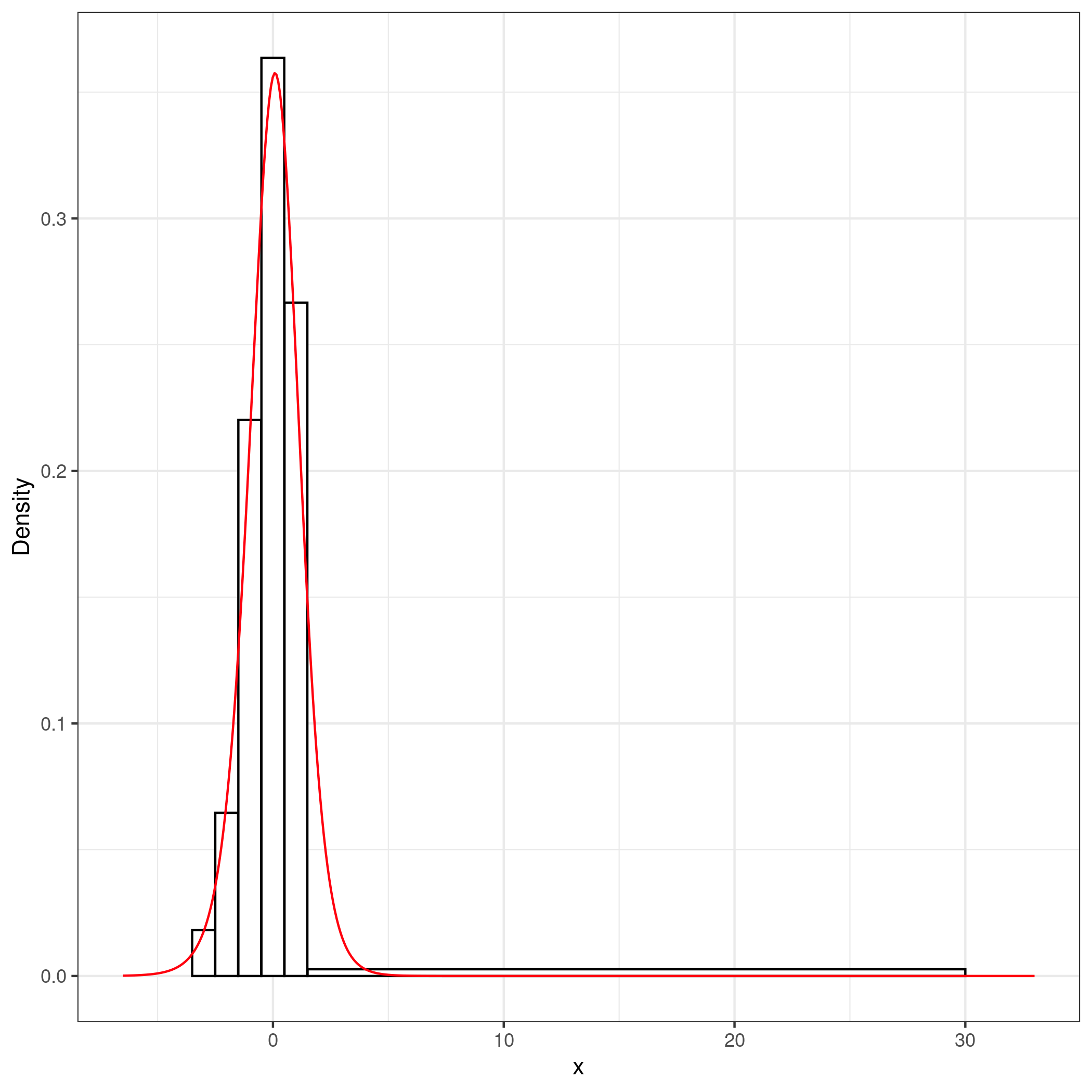
I know this question already received an answer and the results seem really nice (+1)! However I would like to mention also another approach to solve this problem (a similar question was actually asked here). From these frequencies associated to coarse bins, I would estimate the 'implied' density using the penalized composite link histogram smoothing technique proposed in Eilers2007 (in the answer to the question I mentioned above I summarized the main idea behind the approach).

There is a R implementation of this method in the package JOPS. The code below produces a smooth density estimator from your binned data taking the last bin equal to $[1.5, 30]$. You can play with the upper limit if you want. The shape of the fitted density should hardly change (however the shape of the empirical histogram would be affected of course).

I hope this helps and is interesting for you.

library(JOPS)
library(colorout)
library(ggplot2)

# Data
xl  = c(-3.5, -2.5, -1.5, -0.5, 0.5, 1.5) 
xr  = c(-2.51, -1.51, -0.51, 0.49, 1.49, 30)
y   = c(9, 32, 109, 180, 132, 38)

# Set-ups
m    = length(y)
n    = 500
wdts = xr - xl 
dens = y/wdts/sum(y)

# Composition matrix C  1 if finer bin is included in the coarse one, 0 otherwise
x = seq(min(xl)-3, max(xr) + 3, len = n)
C = matrix(0, m, n)
for(i in 1:m) C[i, x >= xl[i] & x <= xr[i]] = 1

# Prepare B-splines bases
B = JOPS::bbase(x, nseg = 30)

# Fit
mod = JOPS::pclm(y, C, B, lambda = 5, pord = 2, show = T)
est = mod$gamma / diff(x)[1] / sum(mod$gamma)

# Plot
fit = data.frame(x = x, fits = est)
dat = data.frame(xl = xl, xr = xr, y = dens)
plt = ggplot(dat, aes(ymin = 0)) + 
geom_rect(aes(xmin = xl, xmax = xr, ymax = y, fill = I('white'), color = I('black'))) +
geom_line(aes(x = x, y = fits), data = fit, col = I('red')) + 
ylab('Density') +
theme_bw()

plt