added 63 characters in body
Source Link
Arya McCarthy
  • 9k
  • 1
  • 24
  • 58

Normalizing flows are often introduced as a way of restricting the rigid priors that are placed on the latent variables in Variational Autoencoders.

For example, from the Pyro docs:

In standard probabilistic modeling practice, we represent our beliefs over unknown continuous quantities with simple parametric distributions like the normal, exponential, and Laplacian distributions. However, using such simple forms, which are commonly symmetric and unimodal (or have a fixed number of modes when we take a mixture of them), restricts the performance and flexibility of our methods.

[...]

Normalizing Flows [1-4] are a family of methods for constructing flexible learnable probability distributions, often with neural networks, which allow us to surpass the limitations of simple parametric forms.

However, it is my understanding that the latent variables $\mathbf{z}$ in normalizing flows are still often modeled as standard Gaussians. For example, the same Pyro docs page gives the following example of a Normalizing Flow:

base_dist = dist.Normal(torch.zeros(2), torch.ones(2))
spline_transform = T.spline_coupling(2, count_bins=16)
flow_dist = dist.TransformedDistribution(base_dist, [spline_transform])

So the base distribution used is a Gaussian, same as in Variational Autoencoders?


To summarize, I have read the statement that normalizing flows somehow "relax" the limitations of Variational Autoencoders, and in particular the limited expressiveness of the latent variable priors that are used, but I am not able to understand why that is the case. Could someone provide a layman explanation and point me to some resources for further reading?

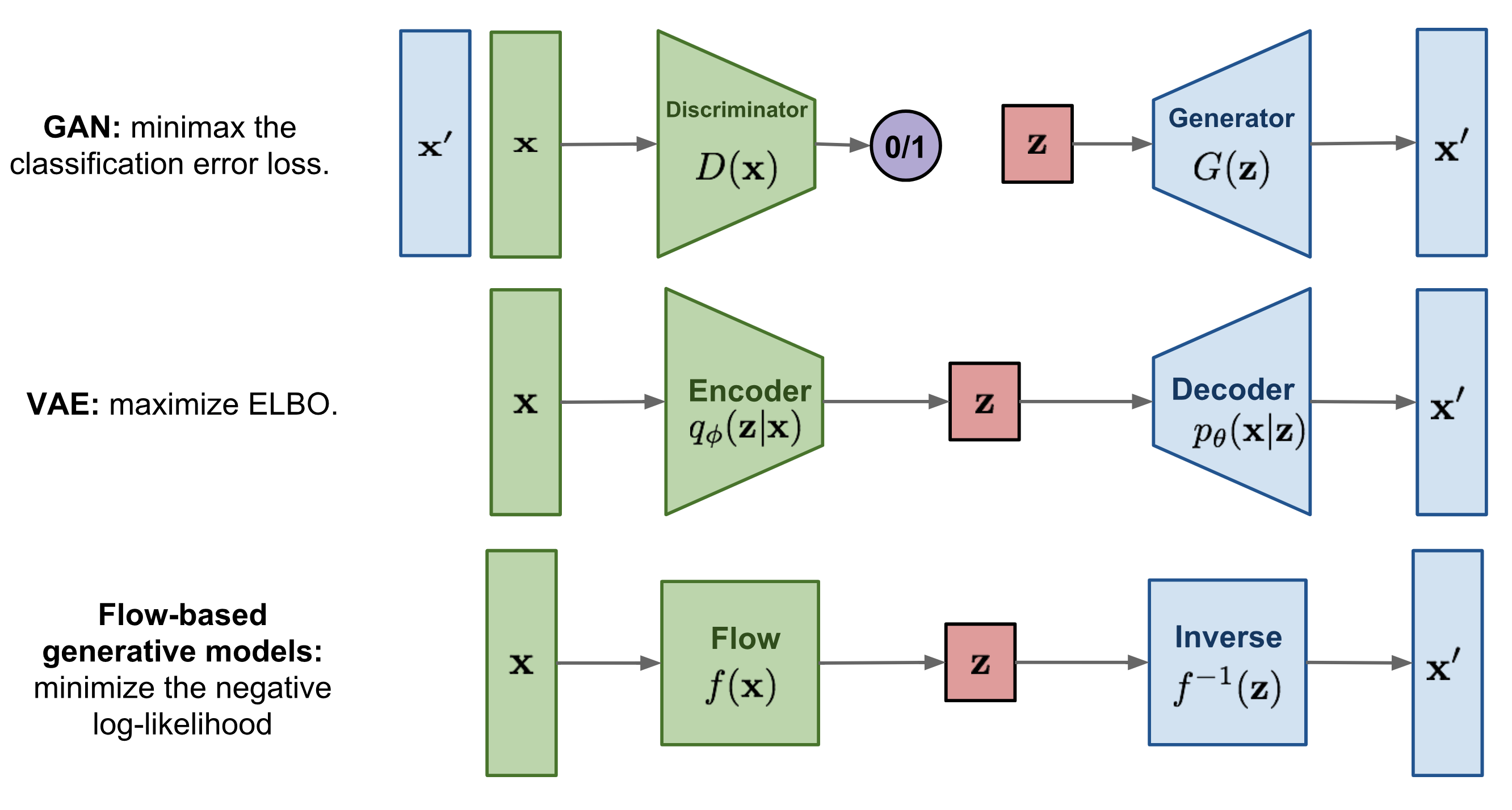
My understanding is that both VAEs and Normalizing Flows map the input $\mathbf{x}$ to some latent representation $\mathbf{z}$ and then attempt to reconstruct the input $\mathbf{\hat{x}}$ from the latent representation. Both VAEs and Normalizing Flows usually model the latent variables $\mathbf{z}$ as coming from independent univariate normal distributions (AFAIK?). Normalizing flows have many more restrictions on the types of neural networks that can be used as the "encoder" and "decoder" (i.e. the model has to be bijective and invertable). So how do normalizing flows relax some of the assumptions of VAEs?

enter image description hereDiagram comparing VAE, GAN, and normalizing flow

Source: https://lilianweng.github.io/lil-log/2018/10/13/flow-based-deep-generative-models.html

Normalizing flows are often introduced as a way of restricting the rigid priors that are placed on the latent variables in Variational Autoencoders.

For example, from the Pyro docs:

In standard probabilistic modeling practice, we represent our beliefs over unknown continuous quantities with simple parametric distributions like the normal, exponential, and Laplacian distributions. However, using such simple forms, which are commonly symmetric and unimodal (or have a fixed number of modes when we take a mixture of them), restricts the performance and flexibility of our methods.

[...]

Normalizing Flows [1-4] are a family of methods for constructing flexible learnable probability distributions, often with neural networks, which allow us to surpass the limitations of simple parametric forms.

However, it is my understanding that the latent variables $\mathbf{z}$ in normalizing flows are still often modeled as standard Gaussians. For example, the same Pyro docs page gives the following example of a Normalizing Flow:

base_dist = dist.Normal(torch.zeros(2), torch.ones(2))
spline_transform = T.spline_coupling(2, count_bins=16)
flow_dist = dist.TransformedDistribution(base_dist, [spline_transform])

So the base distribution used is a Gaussian, same as in Variational Autoencoders?


To summarize, I have read the statement that normalizing flows somehow "relax" the limitations of Variational Autoencoders, and in particular the limited expressiveness of the latent variable priors that are used, but I am not able to understand why that is the case. Could someone provide a layman explanation and point me to some resources for further reading?

My understanding is that both VAEs and Normalizing Flows map the input $\mathbf{x}$ to some latent representation $\mathbf{z}$ and then attempt to reconstruct the input $\mathbf{\hat{x}}$ from the latent representation. Both VAEs and Normalizing Flows usually model the latent variables $\mathbf{z}$ as coming from independent univariate normal distributions (AFAIK?). Normalizing flows have many more restrictions on the types of neural networks that can be used as the "encoder" and "decoder" (i.e. the model has to be bijective and invertable). So how do normalizing flows relax some of the assumptions of VAEs?

enter image description here

Source: https://lilianweng.github.io/lil-log/2018/10/13/flow-based-deep-generative-models.html

Normalizing flows are often introduced as a way of restricting the rigid priors that are placed on the latent variables in Variational Autoencoders.

For example, from the Pyro docs:

In standard probabilistic modeling practice, we represent our beliefs over unknown continuous quantities with simple parametric distributions like the normal, exponential, and Laplacian distributions. However, using such simple forms, which are commonly symmetric and unimodal (or have a fixed number of modes when we take a mixture of them), restricts the performance and flexibility of our methods.

[...]

Normalizing Flows [1-4] are a family of methods for constructing flexible learnable probability distributions, often with neural networks, which allow us to surpass the limitations of simple parametric forms.

However, it is my understanding that the latent variables $\mathbf{z}$ in normalizing flows are still often modeled as standard Gaussians. For example, the same Pyro docs page gives the following example of a Normalizing Flow:

base_dist = dist.Normal(torch.zeros(2), torch.ones(2))
spline_transform = T.spline_coupling(2, count_bins=16)
flow_dist = dist.TransformedDistribution(base_dist, [spline_transform])

So the base distribution used is a Gaussian, same as in Variational Autoencoders?


To summarize, I have read the statement that normalizing flows somehow "relax" the limitations of Variational Autoencoders, and in particular the limited expressiveness of the latent variable priors that are used, but I am not able to understand why that is the case. Could someone provide a layman explanation and point me to some resources for further reading?

My understanding is that both VAEs and Normalizing Flows map the input $\mathbf{x}$ to some latent representation $\mathbf{z}$ and then attempt to reconstruct the input $\mathbf{\hat{x}}$ from the latent representation. Both VAEs and Normalizing Flows usually model the latent variables $\mathbf{z}$ as coming from independent univariate normal distributions (AFAIK?). Normalizing flows have many more restrictions on the types of neural networks that can be used as the "encoder" and "decoder" (i.e. the model has to be bijective and invertable). So how do normalizing flows relax some of the assumptions of VAEs?

Diagram comparing VAE, GAN, and normalizing flow

Source: https://lilianweng.github.io/lil-log/2018/10/13/flow-based-deep-generative-models.html
added 8 characters in body
Source Link
ostrokach
  • 299
  • 3
  • 5

Normalizing flows are often introduced as a way of restricting the rigid priors that are placed on the latent variables in Variational Autoencoders.

For example, from the Pyro docs:

In standard probabilistic modeling practice, we represent our beliefs over unknown continuous quantities with simple parametric distributions like the normal, exponential, and Laplacian distributions. However, using such simple forms, which are commonly symmetric and unimodal (or have a fixed number of modes when we take a mixture of them), restricts the performance and flexibility of our methods.

[...]

Normalizing Flows [1-4] are a family of methods for constructing flexible learnable probability distributions, often with neural networks, which allow us to surpass the limitations of simple parametric forms.

However, it is my understanding that the latent variables $\mathbf{z}$ in normalizing flows are still often modeled as standard Gaussians. For example, the same Pyro docs page gives the following example of a Normalizing Flow:

base_dist = dist.Normal(torch.zeros(2), torch.ones(2))
spline_transform = T.spline_coupling(2, count_bins=16)
flow_dist = dist.TransformedDistribution(base_dist, [spline_transform])

So the base distribution used is a Gaussian, same as in Variational Autoencoders?


To summarize, I have read the statement that normalizing flows somehow "relax" the limitations of Variational Autoencoders, and in particular the limited expressiveness of the latent variable priors that are used, but I am not able to understand why that is the case. Could someone provide a layman explanation and point me to some resources for further reading?

My understanding is that both VAEs and Normalizing Flows map the input $\mathbf{x}$ to some latent representation $\mathbf{z}$ and then attempt to reconstruct the input $\mathbf{\hat{x}}$ from the latent representation. Both VAEs and Normalizing Flows usually model the latent variables $\mathbf{z}$ as coming from independent univariate normal distributions (AFAIK?). Normalizing flows have many more restrictions on the types of neural networks that can be used as the "encoder" and "decoder" (i.e. the model has to be bijective and we need to be able to calculate the determinant of the Jacobianinvertable). So how do normalizing flows relax some of the assumptions of VAEs?

enter image description here

Source: https://lilianweng.github.io/lil-log/2018/10/13/flow-based-deep-generative-models.html

Normalizing flows are often introduced as a way of restricting the rigid priors that are placed on the latent variables in Variational Autoencoders.

For example, from the Pyro docs:

In standard probabilistic modeling practice, we represent our beliefs over unknown continuous quantities with simple parametric distributions like the normal, exponential, and Laplacian distributions. However, using such simple forms, which are commonly symmetric and unimodal (or have a fixed number of modes when we take a mixture of them), restricts the performance and flexibility of our methods.

[...]

Normalizing Flows [1-4] are a family of methods for constructing flexible learnable probability distributions, often with neural networks, which allow us to surpass the limitations of simple parametric forms.

However, it is my understanding that the latent variables $\mathbf{z}$ in normalizing flows are still often as standard Gaussians. For example, the same Pyro docs page gives the following example of a Normalizing Flow:

base_dist = dist.Normal(torch.zeros(2), torch.ones(2))
spline_transform = T.spline_coupling(2, count_bins=16)
flow_dist = dist.TransformedDistribution(base_dist, [spline_transform])

So the base distribution used is a Gaussian, same as in Variational Autoencoders?


To summarize, I have read the statement that normalizing flows somehow "relax" the limitations of Variational Autoencoders, and in particular the limited expressiveness of the latent variable priors that are used, but I am not able to understand why that is the case. Could someone provide a layman explanation and point me to some resources for further reading?

My understanding is that both VAEs and Normalizing Flows map the input $\mathbf{x}$ to some latent representation $\mathbf{z}$ and then attempt to reconstruct the input $\mathbf{\hat{x}}$ from the latent representation. Both VAEs and Normalizing Flows usually model the latent variables $\mathbf{z}$ as independent univariate normal distributions (AFAIK?). Normalizing flows have many more restrictions on the types of neural networks that can be used as the "encoder" and "decoder" (i.e. the model has to be bijective and we need to be able to calculate the determinant of the Jacobian). So how do normalizing flows relax some of the assumptions of VAEs?

enter image description here

Source: https://lilianweng.github.io/lil-log/2018/10/13/flow-based-deep-generative-models.html

Normalizing flows are often introduced as a way of restricting the rigid priors that are placed on the latent variables in Variational Autoencoders.

For example, from the Pyro docs:

In standard probabilistic modeling practice, we represent our beliefs over unknown continuous quantities with simple parametric distributions like the normal, exponential, and Laplacian distributions. However, using such simple forms, which are commonly symmetric and unimodal (or have a fixed number of modes when we take a mixture of them), restricts the performance and flexibility of our methods.

[...]

Normalizing Flows [1-4] are a family of methods for constructing flexible learnable probability distributions, often with neural networks, which allow us to surpass the limitations of simple parametric forms.

However, it is my understanding that the latent variables $\mathbf{z}$ in normalizing flows are still often modeled as standard Gaussians. For example, the same Pyro docs page gives the following example of a Normalizing Flow:

base_dist = dist.Normal(torch.zeros(2), torch.ones(2))
spline_transform = T.spline_coupling(2, count_bins=16)
flow_dist = dist.TransformedDistribution(base_dist, [spline_transform])

So the base distribution used is a Gaussian, same as in Variational Autoencoders?


To summarize, I have read the statement that normalizing flows somehow "relax" the limitations of Variational Autoencoders, and in particular the limited expressiveness of the latent variable priors that are used, but I am not able to understand why that is the case. Could someone provide a layman explanation and point me to some resources for further reading?

My understanding is that both VAEs and Normalizing Flows map the input $\mathbf{x}$ to some latent representation $\mathbf{z}$ and then attempt to reconstruct the input $\mathbf{\hat{x}}$ from the latent representation. Both VAEs and Normalizing Flows usually model the latent variables $\mathbf{z}$ as coming from independent univariate normal distributions (AFAIK?). Normalizing flows have many more restrictions on the types of neural networks that can be used as the "encoder" and "decoder" (i.e. the model has to be bijective and invertable). So how do normalizing flows relax some of the assumptions of VAEs?

enter image description here

Source: https://lilianweng.github.io/lil-log/2018/10/13/flow-based-deep-generative-models.html

added 846 characters in body
Source Link
ostrokach
  • 299
  • 3
  • 5

Normalizing flows are often introduced as a way of restricting the rigid priors that are placed on the latent variables in Variational Autoencoders.

For example, from the Pyro docs:

In standard probabilistic modeling practice, we represent our beliefs over unknown continuous quantities with simple parametric distributions like the normal, exponential, and Laplacian distributions. However, using such simple forms, which are commonly symmetric and unimodal (or have a fixed number of modes when we take a mixture of them), restricts the performance and flexibility of our methods.

[...]

Normalizing Flows [1-4] are a family of methods for constructing flexible learnable probability distributions, often with neural networks, which allow us to surpass the limitations of simple parametric forms.

However, it is my understanding that the latent variables $\mathbf{z}$ in normalizing flows are still often as standard Gaussians. For example, the same Pyro docs page gives the following example of a Normalizing Flow:

base_dist = dist.Normal(torch.zeros(2), torch.ones(2))
spline_transform = T.spline_coupling(2, count_bins=16)
flow_dist = dist.TransformedDistribution(base_dist, [spline_transform])

So the base distribution used is a Gaussian, same as in Variational Autoencoders?


To summarize, I have read the statement that normalizing flows somehow "relax" the limitations of Variational Autoencoders, and in particular the limited expressiveness of the latent variable priors that are used, but I am not able to understand why that is the case. Could someone provide a layman explanation and point me to some resources for further reading?

My understanding is that both VAEs and Normalizing Flows map the input $\mathbf{x}$ to some latent representation $\mathbf{z}$ and then attempt to reconstruct the input $\mathbf{\hat{x}}$ from the latent representation. Both VAEs and Normalizing Flows usually model the latent variables $\mathbf{z}$ as independent univariate normal distributions (AFAIK?). Normalizing flows have many more restrictions on the types of neural networks that can be used as the "encoder" and "decoder" (i.e. the model has to be bijective and we need to be able to calculate the determinant of the Jacobian). So how do normalizing flows relax some of the assumptions of VAEs?

enter image description here

Source: https://lilianweng.github.io/lil-log/2018/10/13/flow-based-deep-generative-models.html

Normalizing flows are often introduced as a way of restricting the rigid priors that are placed on the latent variables in Variational Autoencoders.

For example, from the Pyro docs:

In standard probabilistic modeling practice, we represent our beliefs over unknown continuous quantities with simple parametric distributions like the normal, exponential, and Laplacian distributions. However, using such simple forms, which are commonly symmetric and unimodal (or have a fixed number of modes when we take a mixture of them), restricts the performance and flexibility of our methods.

[...]

Normalizing Flows [1-4] are a family of methods for constructing flexible learnable probability distributions, often with neural networks, which allow us to surpass the limitations of simple parametric forms.

However, it is my understanding that the latent variables $\mathbf{z}$ in normalizing flows are still often as standard Gaussians. For example, the same Pyro docs page gives the following example of a Normalizing Flow:

base_dist = dist.Normal(torch.zeros(2), torch.ones(2))
spline_transform = T.spline_coupling(2, count_bins=16)
flow_dist = dist.TransformedDistribution(base_dist, [spline_transform])

So the base distribution used is a Gaussian, same as in Variational Autoencoders?

To summarize, I have read the statement that normalizing flows somehow "relax" the limitations of Variational Autoencoders, and in particular the limited expressiveness of the latent variable priors that are used, but I am not able to understand why that is the case. Could someone provide a layman explanation and point me to some resources for further reading?

Normalizing flows are often introduced as a way of restricting the rigid priors that are placed on the latent variables in Variational Autoencoders.

For example, from the Pyro docs:

In standard probabilistic modeling practice, we represent our beliefs over unknown continuous quantities with simple parametric distributions like the normal, exponential, and Laplacian distributions. However, using such simple forms, which are commonly symmetric and unimodal (or have a fixed number of modes when we take a mixture of them), restricts the performance and flexibility of our methods.

[...]

Normalizing Flows [1-4] are a family of methods for constructing flexible learnable probability distributions, often with neural networks, which allow us to surpass the limitations of simple parametric forms.

However, it is my understanding that the latent variables $\mathbf{z}$ in normalizing flows are still often as standard Gaussians. For example, the same Pyro docs page gives the following example of a Normalizing Flow:

base_dist = dist.Normal(torch.zeros(2), torch.ones(2))
spline_transform = T.spline_coupling(2, count_bins=16)
flow_dist = dist.TransformedDistribution(base_dist, [spline_transform])

So the base distribution used is a Gaussian, same as in Variational Autoencoders?


To summarize, I have read the statement that normalizing flows somehow "relax" the limitations of Variational Autoencoders, and in particular the limited expressiveness of the latent variable priors that are used, but I am not able to understand why that is the case. Could someone provide a layman explanation and point me to some resources for further reading?

My understanding is that both VAEs and Normalizing Flows map the input $\mathbf{x}$ to some latent representation $\mathbf{z}$ and then attempt to reconstruct the input $\mathbf{\hat{x}}$ from the latent representation. Both VAEs and Normalizing Flows usually model the latent variables $\mathbf{z}$ as independent univariate normal distributions (AFAIK?). Normalizing flows have many more restrictions on the types of neural networks that can be used as the "encoder" and "decoder" (i.e. the model has to be bijective and we need to be able to calculate the determinant of the Jacobian). So how do normalizing flows relax some of the assumptions of VAEs?

enter image description here

Source: https://lilianweng.github.io/lil-log/2018/10/13/flow-based-deep-generative-models.html

Source Link
ostrokach
  • 299
  • 3
  • 5
Loading