edited body
Source Link
Ben
  • 132.9k
  • 7
  • 255
  • 588

One final thing that is worth noting in relation to this issue is that a classical hypothesis test is essentially an inductive analogue to the deductive proof by contradiction (see related answers here and here). In a proof by contradiction we begin with a null hypothesis, show that this leads logically to a contradiction, and therefore reject the initial premise that the null is true (with certainty). In a classical hypothesis test, we begin with a null hypothesis, show that this leads to a highly implausible result in favour of the alternative (so not quite a deductive contradiction, but close), and therefore reject the initial premise that the null is true (but with some uncertainty). The p-value in this test is the probability of a result at least as conducive to the alternative hypothesis, assuming the null is true. If this is low then it means that something very implausible happened (under the assumption that the null is true) which gives the "contradiction" in the "inductive proof by contradiction". Just as with a proof by contradiction, this procedure is asymmetric in the hypotheses and it is only necessary to look at things conditional on the null hypothesis. THe The alternative hypothesis contributes only to the extent that it helps us understand what is a more implausible result under the null hypothesis (i.e., through the evidentiary ordering) which allows us to inductively measure the "implausibility" that is analogous to a contradiction.

One final thing that is worth noting in relation to this issue is that a classical hypothesis test is essentially an inductive analogue to the deductive proof by contradiction (see related answers here and here). In a proof by contradiction we begin with a null hypothesis, show that this leads logically to a contradiction, and therefore reject the initial premise that the null is true (with certainty). In a classical hypothesis test, we begin with a null hypothesis, show that this leads to a highly implausible result in favour of the alternative (so not quite a deductive contradiction, but close), and therefore reject the initial premise that the null is true (but with some uncertainty). The p-value in this test is the probability of a result at least as conducive to the alternative hypothesis, assuming the null is true. If this is low then it means that something very implausible happened (under the assumption that the null is true) which gives the "contradiction" in the "inductive proof by contradiction". Just as with a proof by contradiction, this procedure is asymmetric in the hypotheses and it is only necessary to look at things conditional on the null hypothesis. THe alternative hypothesis contributes only to the extent that it helps us understand what is a more implausible result under the null hypothesis (i.e., through the evidentiary ordering) which allows us to inductively measure the "implausibility" that is analogous to a contradiction.

One final thing that is worth noting in relation to this issue is that a classical hypothesis test is essentially an inductive analogue to the deductive proof by contradiction (see related answers here and here). In a proof by contradiction we begin with a null hypothesis, show that this leads logically to a contradiction, and therefore reject the initial premise that the null is true (with certainty). In a classical hypothesis test, we begin with a null hypothesis, show that this leads to a highly implausible result in favour of the alternative (so not quite a deductive contradiction, but close), and therefore reject the initial premise that the null is true (but with some uncertainty). The p-value in this test is the probability of a result at least as conducive to the alternative hypothesis, assuming the null is true. If this is low then it means that something very implausible happened (under the assumption that the null is true) which gives the "contradiction" in the "inductive proof by contradiction". Just as with a proof by contradiction, this procedure is asymmetric in the hypotheses and it is only necessary to look at things conditional on the null hypothesis. The alternative hypothesis contributes only to the extent that it helps us understand what is a more implausible result under the null hypothesis (i.e., through the evidentiary ordering) which allows us to inductively measure the "implausibility" that is analogous to a contradiction.

added 256 characters in body
Source Link
Ben
  • 132.9k
  • 7
  • 255
  • 588

One final thing that is worth noting in relation to this issue is that a classical hypothesis test is essentially an inductive analogue to the deductive proof by contradiction (see related answers here and here). In a proof by contradiction we begin with a null hypothesis, show that this leads logically to a contradiction, and therefore reject the initial premise that the null is true (with certainty). In a classical hypothesis test, we begin with a null hypothesis, show that this leads to a highly implausible result in favour of the alternative (so not quite a deductive contradiction, but close), and therefore reject the initial premise that the null is true (but with some uncertainty). The p-value in this test is the probability of a result at least as conducive to the alternative hypothesis, assuming the null is true. If this is low then it means that something very implausible happened (under the assumption that the null is true) which gives the "contradiction" in the "inductive proof by contradiction". Just as with a proof by contradiction, this procedure is asymmetric in the hypotheses and it is only necessary to look at things conditional on the null hypothesis. THe alternative hypothesis contributes only to the extent that it helps us understand what is a more implausible result under the null hypothesis (i.e., through the evidentiary ordering) which allows us to inductively measure the "implausibility" that is analogous to a contradiction.

One final thing that is worth noting in relation to this issue is that a classical hypothesis test is essentially an inductive analogue to the deductive proof by contradiction (see related answers here and here). In a proof by contradiction we begin with a null hypothesis, show that this leads logically to a contradiction, and therefore reject the initial premise that the null is true (with certainty). In a classical hypothesis test, we begin with a null hypothesis, show that this leads to a highly implausible result in favour of the alternative (so not quite a deductive contradiction, but close), and therefore reject the initial premise that the null is true (but with some uncertainty). The p-value in this test is the probability of a result at least as conducive to the alternative hypothesis, assuming the null is true. If this is low then it means that something very implausible happened (under the assumption that the null is true) which gives the "contradiction" in the "inductive proof by contradiction". Just as with a proof by contradiction, this procedure is asymmetric in the hypotheses and it is only necessary to look at things conditional on the null hypothesis. THe alternative hypothesis contributes only to the extent that it helps us understand what is a more implausible result under the null hypothesis (i.e., through the evidentiary ordering) which allows us to inductively measure the "implausibility" that is analogous to a contradiction.

added 256 characters in body
Source Link
Ben
  • 132.9k
  • 7
  • 255
  • 588

The alternative hypothesis affects the test through the evidentiary ordering

The p-value of a classical hypothesis test depends on the alternative hypothesis only through the evidentiary ordering constructed for the test, which is what tells you what constitutes an "extreme" observation. Any hypothesis test involves specification of an evidentiary ordering which is a total preorder on the set of all possible outcomes of the observable data. This evidentiary ordering specifies which outcomes are more conducive to the null or alternative hypotheses respectively. Often this ordering is implicit on having defined a "test statistic" for the test, but the only role of the test statistic is to represent this ordering.


Hypothesis testing via an evidentiary ordering: Suppose we want to create a hypothesis test for an unknown parameter $\theta \in \Theta$ using an observable random vector $\mathbf{X} \in \mathscr{X}$ with a distribution that depends on this parameter. For any stipulated null space $\Theta_0$ and alternative space $\Theta_A$ (and any particular logic for how the test works) we contruct a total preorder $\succeq$ on the outcome space $\mathscr{X}$. The interpretation of the total preorder is:

$$\mathbf{x} \succeq \mathbf{x}' \quad \quad \iff \quad \quad \mathbf{x} \text{ is at least as conducive to } H_A \text{ as } \mathbf{x}'.$$

For brevity, we sometimes say that $\mathbf{x} \succeq \mathbf{x}'$ means that $\mathbf{x}$ is at least as "extreme" as $\mathbf{x}'$. This is a common shorthand, which is okay if you remember that "extreme" means "conducive to the alternative hypothesis" in this context. In practice, the evidentiary ordering for the sample space is often set implicitly by constructing a test statistic and having an ordering for the test statistic.$^\dagger$ This is essentially just the same thing, but removed one-level of abstraction away from the sample space in order to conentrateconcentrate entirely on the ordering.

You should bear in mind that the situation is complicated slightly by the fact that the "test statistic" and "evidentiary ordering" may both be dependent on the parameter in the analysis. In fact, the "test statistic" is typically not a statistic, but often instead a pivotal quantity that depends on the parameter value in the hypothesis. In this case the evidentiary ordering will also be implicitly dependent on the parameter. (In the case of a test with a simple null hypothesis this doesn't matter, because the test always conditions on this single value. In the case of a test with a composite hypothesis it might matter, because the ordering now changes over the null space.) Taking this dependence as implicit for now, once we have set the evidentiary ordering for the test, the p-value function is then defined as:

$$p(\mathbf{x}) \equiv \sup_{\theta \in \Theta_0} \mathbb{P}(\mathbf{X} \succeq \mathbf{x} | \theta) \quad \quad \quad \text{for all } \mathbf{x} \in \mathscr{X}.$$

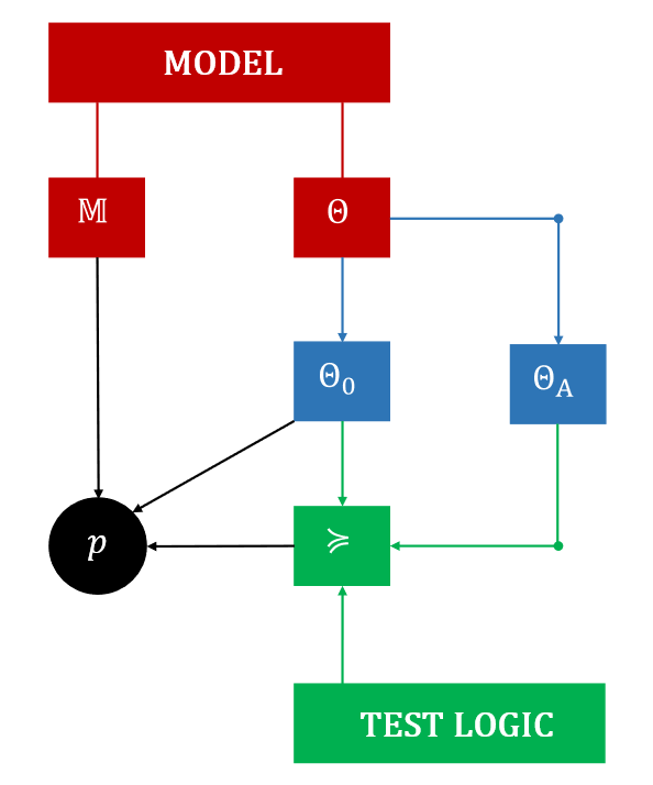
If we denote the probabilistic model by $\mathbb{M} \equiv \{ \mathbb{P}(\cdot | \theta) | \theta \in \Theta \}$ then we can write the p-value function as a function $p = f(\mathbb{M}, \Theta_0, \succeq)$. We can see that the p-value function is fully determined by the model $\mathbb{M}$, the null space $\Theta_0$ and the evidentiary ordering $\succeq$. Observe that the alternative hypothesis only affects this function through its contribution to the evidentiary ordering.

The structure of a classical hypothesis test is shown in the diagram below. This diagram illustrates the elements of the test that lead to the p-value function, which ultimately defines the test. As can be seen in the diagram, the alternative hypothesis has a limited role; combined with the logic of the test it affects the evidentiary ordering for the test, which then flows into determination of the p-value function.
enter image description here


$^\dagger$ Often the evidentiary ordering is set implicitly using a test statistic $T: \mathscr{X} \rightarrow \mathbb{R}$ and then using the ordering defined by the correspondence $\mathbf{x}_0 \succeq \mathbf{x}_1 \iff T(\mathbf{x}_0) \geqslant T(\mathbf{x}_1)$. In this case the p-value reduces to $p(\mathbf{x}) = \sup_{\theta \in \Theta_0} \mathbb{P}(T(\mathbf{X}) \geqslant T(\mathbf{x}) | \theta)$.

The alternative hypothesis affects the test through the evidentiary ordering

The p-value of a classical hypothesis test depends on the alternative hypothesis only through the evidentiary ordering constructed for the test, which is what tells you what constitutes an "extreme" observation. Any hypothesis test involves specification of an evidentiary ordering which is a total preorder on the set of all possible outcomes of the observable data. This evidentiary ordering specifies which outcomes are more conducive to the null or alternative hypotheses respectively. Often this ordering is implicit on having defined a "test statistic" for the test, but the only role of the test statistic is to represent this ordering.


Hypothesis testing via an evidentiary ordering: Suppose we want to create a hypothesis test for an unknown parameter $\theta \in \Theta$ using an observable random vector $\mathbf{X} \in \mathscr{X}$ with a distribution that depends on this parameter. For any stipulated null space $\Theta_0$ and alternative space $\Theta_A$ (and any particular logic for how the test works) we contruct a total preorder $\succeq$ on the outcome space $\mathscr{X}$. The interpretation of the total preorder is:

$$\mathbf{x} \succeq \mathbf{x}' \quad \quad \iff \quad \quad \mathbf{x} \text{ is at least as conducive to } H_A \text{ as } \mathbf{x}'.$$

For brevity, we sometimes say that $\mathbf{x} \succeq \mathbf{x}'$ means that $\mathbf{x}$ is at least as "extreme" as $\mathbf{x}'$. This is a common shorthand, which is okay if you remember that "extreme" means "conducive to the alternative hypothesis" in this context. In practice, the evidentiary ordering for the sample space is often set implicitly by constructing a test statistic and having an ordering for the test statistic.$^\dagger$ This is essentially just the same thing, but removed one-level of abstraction away from the sample space in order to conentrate entirely on the ordering.

You should bear in mind that the situation is complicated slightly by the fact that the "test statistic" and "evidentiary ordering" may both be dependent on the parameter in the analysis. In fact, the "test statistic" is typically not a statistic, but often instead a pivotal quantity that depends on the parameter value in the hypothesis. In this case the evidentiary ordering will also be implicitly dependent on the parameter. Taking this dependence as implicit for now, once we have set the evidentiary ordering for the test, the p-value function is then defined as:

$$p(\mathbf{x}) \equiv \sup_{\theta \in \Theta_0} \mathbb{P}(\mathbf{X} \succeq \mathbf{x} | \theta) \quad \quad \quad \text{for all } \mathbf{x} \in \mathscr{X}.$$

If we denote the probabilistic model by $\mathbb{M} \equiv \{ \mathbb{P}(\cdot | \theta) | \theta \in \Theta \}$ then we can write the p-value function as a function $p = f(\mathbb{M}, \Theta_0, \succeq)$. We can see that the p-value function is fully determined by the model $\mathbb{M}$, the null space $\Theta_0$ and the evidentiary ordering $\succeq$. Observe that the alternative hypothesis only affects this function through its contribution to the evidentiary ordering.

The structure of a classical hypothesis test is shown in the diagram below. This diagram illustrates the elements of the test that lead to the p-value function, which ultimately defines the test. As can be seen in the diagram, the alternative hypothesis has a limited role; combined with the logic of the test it affects the evidentiary ordering for the test, which then flows into determination of the p-value function.

enter image description here


$^\dagger$ Often the evidentiary ordering is set implicitly using a test statistic $T: \mathscr{X} \rightarrow \mathbb{R}$ and then using the ordering defined by the correspondence $\mathbf{x}_0 \succeq \mathbf{x}_1 \iff T(\mathbf{x}_0) \geqslant T(\mathbf{x}_1)$. In this case the p-value reduces to $p(\mathbf{x}) = \sup_{\theta \in \Theta_0} \mathbb{P}(T(\mathbf{X}) \geqslant T(\mathbf{x}) | \theta)$.

The alternative hypothesis affects the test through the evidentiary ordering

The p-value of a classical hypothesis test depends on the alternative hypothesis only through the evidentiary ordering constructed for the test, which is what tells you what constitutes an "extreme" observation. Any hypothesis test involves specification of an evidentiary ordering which is a total preorder on the set of all possible outcomes of the observable data. This evidentiary ordering specifies which outcomes are more conducive to the null or alternative hypotheses respectively. Often this ordering is implicit on having defined a "test statistic" for the test, but the only role of the test statistic is to represent this ordering.


Hypothesis testing via an evidentiary ordering: Suppose we want to create a hypothesis test for an unknown parameter $\theta \in \Theta$ using an observable random vector $\mathbf{X} \in \mathscr{X}$ with a distribution that depends on this parameter. For any stipulated null space $\Theta_0$ and alternative space $\Theta_A$ (and any particular logic for how the test works) we contruct a total preorder $\succeq$ on the outcome space $\mathscr{X}$. The interpretation of the total preorder is:

$$\mathbf{x} \succeq \mathbf{x}' \quad \quad \iff \quad \quad \mathbf{x} \text{ is at least as conducive to } H_A \text{ as } \mathbf{x}'.$$

For brevity, we sometimes say that $\mathbf{x} \succeq \mathbf{x}'$ means that $\mathbf{x}$ is at least as "extreme" as $\mathbf{x}'$. This is a common shorthand, which is okay if you remember that "extreme" means "conducive to the alternative hypothesis" in this context. In practice, the evidentiary ordering for the sample space is often set implicitly by constructing a test statistic and having an ordering for the test statistic.$^\dagger$ This is essentially just the same thing, but removed one-level of abstraction away from the sample space in order to concentrate entirely on the ordering.

You should bear in mind that the situation is complicated slightly by the fact that the "test statistic" and "evidentiary ordering" may both be dependent on the parameter in the analysis. In fact, the "test statistic" is typically not a statistic, but often instead a pivotal quantity that depends on the parameter value in the hypothesis. In this case the evidentiary ordering will also be implicitly dependent on the parameter. (In the case of a test with a simple null hypothesis this doesn't matter, because the test always conditions on this single value. In the case of a test with a composite hypothesis it might matter, because the ordering now changes over the null space.) Taking this dependence as implicit for now, once we have set the evidentiary ordering for the test, the p-value function is then defined as:

$$p(\mathbf{x}) \equiv \sup_{\theta \in \Theta_0} \mathbb{P}(\mathbf{X} \succeq \mathbf{x} | \theta) \quad \quad \quad \text{for all } \mathbf{x} \in \mathscr{X}.$$

If we denote the probabilistic model by $\mathbb{M} \equiv \{ \mathbb{P}(\cdot | \theta) | \theta \in \Theta \}$ then we can write the p-value function as a function $p = f(\mathbb{M}, \Theta_0, \succeq)$. We can see that the p-value function is fully determined by the model $\mathbb{M}$, the null space $\Theta_0$ and the evidentiary ordering $\succeq$. Observe that the alternative hypothesis only affects this function through its contribution to the evidentiary ordering.

The structure of a classical hypothesis test is shown in the diagram below. This diagram illustrates the elements of the test that lead to the p-value function, which ultimately defines the test. As can be seen in the diagram, the alternative hypothesis has a limited role; combined with the logic of the test it affects the evidentiary ordering for the test, which then flows into determination of the p-value function.

enter image description here


$^\dagger$ Often the evidentiary ordering is set implicitly using a test statistic $T: \mathscr{X} \rightarrow \mathbb{R}$ and then using the ordering defined by the correspondence $\mathbf{x}_0 \succeq \mathbf{x}_1 \iff T(\mathbf{x}_0) \geqslant T(\mathbf{x}_1)$. In this case the p-value reduces to $p(\mathbf{x}) = \sup_{\theta \in \Theta_0} \mathbb{P}(T(\mathbf{X}) \geqslant T(\mathbf{x}) | \theta)$.

added 534 characters in body
Source Link
Ben
  • 132.9k
  • 7
  • 255
  • 588
Loading
deleted 6 characters in body
Source Link
User1865345
  • 10.3k
  • 12
  • 23
  • 40
Loading
added 66 characters in body
Source Link
Ben
  • 132.9k
  • 7
  • 255
  • 588
Loading
Added diagram
Source Link
Ben
  • 132.9k
  • 7
  • 255
  • 588
Loading
deleted 2 characters in body
Source Link
Ben
  • 132.9k
  • 7
  • 255
  • 588
Loading
added 1 character in body
Source Link
Ben
  • 132.9k
  • 7
  • 255
  • 588
Loading
Source Link
Ben
  • 132.9k
  • 7
  • 255
  • 588
Loading