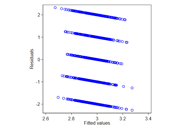
This answer focuses on the second question, generalized to Why do I get striping in my residuals? That question often arises in one form or another. The surprise people have on spotting such patterns is, one hopes, matched by the pleasure of understanding them when the reason is explained. The answer is generic to any plot of residuals versus fitted or predicted values, whenever the definition is the usual or default form
residual = observed $-$ fitted.
It follows easily from the definition that instances of each distinct value of the observed lie on a straight line with gradient $-1$, namely
residual = this observed value $-$ fitted,
as they have the same observed value but typically different fitted values given often different values on corresponding predictors.
If the observed values are all or mostly distinct, then that will still be true but not obvious as striping on a mere scatter plot. However, if
- Observed values are bounded sharply or nearly, limiting lines may be discernible either because data lie on but not beyond those lines or because a limit may be traced by eye. Simple examples are
(a) when observed values must be positive, or positive or zero, and the smallest values are zero on, or at least close to zero;
(b) when values are proportions or percents in [0, 1]$[0, 1]$ or [0, 100];$[0, 100]$;
(c) with binary outcomes 0$0$ or 1$1$ (although in this case the effect does not usually cause surprise and it is widely known that better plots should be used).
- If there is a small set of distinct values, they will define a discernible set of parallel lines. Simple examples are
(d) counts, especially when most data are small counts;
(e) Likert-type ordinal scores fitted with a linear model.
Other definitions of residual don't all undermine this phenomenon, which may still be detectable in modified form.
The explanation should come with at least one graphical example. Here is a nonsense model in which scores 1$1$ to 5$5$ are from a discrete uniform and modelled withthe model includes a predictor that is Gaussian noise. The pattern on the residual versus fitted plot is thus pure artefact.
For the record, here is the Stata code used, which could be matched by code in any other statistical or mathematical software:
clear
set obs 1000
set seed 314159265
set scheme s1color

gen y = runiformint(1, 5)
gen x = rnormal()

regress y x
rvfplot, ms(Oh) mc(blue) yla(, ang(h)) aspect(1)

