added 266 characters in body
Source Link
Sextus Empiricus
  • 86.6k
  • 6
  • 115
  • 304

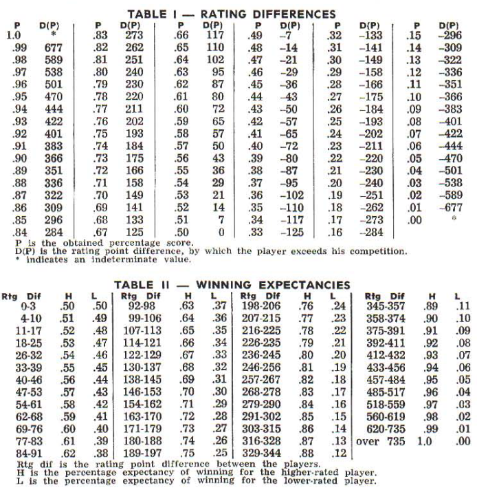
Below we see the specific tables from Elo, Arpad E. (August, 1967). The Proposed USCF Rating System, Its Development, Theory, and Applications. Chess Life XXII (8): 242-247.

copy of tables

The values in table I seem to be an average of the values in table II (rather than a direct computation with the quantile function).

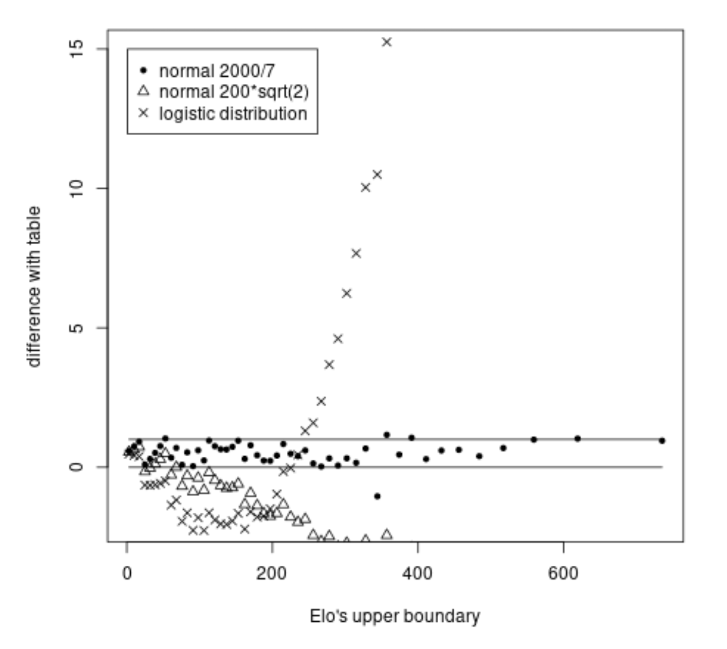
The values in table II correspond very well with a normal distribution that has standard deviation $2000/7$. The upper boundaries will be equal to the percentile scores of the normal distribution rounded down and the lower boundaries will be equal to the percentile scores of the normal distribution rounded up. Below you see a comparison of three methods.

example

The logistic distribution or a normal distribution with standard deviation $200 \sqrt{2}$ have large differences.

For the normal distribution with standard deviation $2000/7$ there are some small discrepancies, but only of the order of $\pm 1$ and that can be due to round-off errors and use of tables with lower precision* or possibly a typo.

p = seq(0.505,0.995,0.01)
elo1 = qnorm(p,0,2000/7)
elo2 = qnorm(p,0,200*sqrt(2))
elo3 = -log10(1/p-1)*400

x = c(3,10,17,25,32,39,46,53,61,68,76,83,91,98,106,113,121,129,137,145,153,162,170,179,188,197,206,215,225,235,245,256,267,278,290,302,315,328,344,357,374,391,411,432,456,484,517,559,619,735)

plot(x,x-x, type = "l", xlab = "Elo's upper boundary", log = "", ylim = c(-2,15), ylab = "difference with table")
points(x,elo1-x, pch = 20)
points(x,elo2-x, pch = 2)
points(x,elo3-x, pch = 4)

legend(1,15, c("normal 2000/7", "normal 200*sqrt(2)", "logistic distribution"), cex = 1, pch = c(20,2,4))

lines(x,x*0+1)

In 'The rating of chess players, past and present' Elo writes an example

For example. let D = 160. Then z = 160/282.84 = .566. The table gives .7143 and .2857 as the areas of the two portions under the curve. These probabilities are rounded to two figures in table 2.11

This suggests that he used sufficiently accurate tables with at least 4 figures. An example could be Table X (copied from Pearson) in Garrett's 'statistics in psychology and education' which occurs as a reference.
Below we see the specific tables from Elo, Arpad E. (August, 1967). The Proposed USCF Rating System, Its Development, Theory, and Applications. Chess Life XXII (8): 242-247.

copy of tables

The values in table I seem to be an average of the values in table II (rather than a direct computation with the quantile function).

The values in table II correspond very well with a normal distribution that has standard deviation $2000/7$. The upper boundaries will be equal to the percentile scores of the normal distribution rounded down and the lower boundaries will be equal to the percentile scores of the normal distribution rounded up. Below you see a comparison of three methods.

example

The logistic distribution or a normal distribution with standard deviation $200 \sqrt{2}$ have large differences.

For the normal distribution with standard deviation $2000/7$ there are some small discrepancies, but only of the order of $\pm 1$ and that can be due to round-off errors and use of tables with lower precision* or possibly a typo.

p = seq(0.505,0.995,0.01)
elo1 = qnorm(p,0,2000/7)
elo2 = qnorm(p,0,200*sqrt(2))
elo3 = -log10(1/p-1)*400

x = c(3,10,17,25,32,39,46,53,61,68,76,83,91,98,106,113,121,129,137,145,153,162,170,179,188,197,206,215,225,235,245,256,267,278,290,302,315,328,344,357,374,391,411,432,456,484,517,559,619,735)

plot(x,x-x, type = "l", xlab = "Elo's upper boundary", log = "", ylim = c(-2,15), ylab = "difference with table")
points(x,elo1-x, pch = 20)
points(x,elo2-x, pch = 2)
points(x,elo3-x, pch = 4)

legend(1,15, c("normal 2000/7", "normal 200*sqrt(2)", "logistic distribution"), cex = 1, pch = c(20,2,4))

lines(x,x*0+1)

In 'The rating of chess players, past and present' Elo writes an example

For example. let D = 160. Then z = 160/282.84 = .566. The table gives .7143 and .2857 as the areas of the two portions under the curve. These probabilities are rounded to two figures in table 2.11

This suggests that he used sufficiently accurate tables with at least 4 figures. An example could be Table X (copied from Pearson) in Garrett's 'statistics in psychology and education' which occurs as a reference.

added 514 characters in body
Source Link
Sextus Empiricus
  • 86.6k
  • 6
  • 115
  • 304

copy of tables

The values in table I seem to be an average of the values in table II (rather than a direct computation with the quantile function).

The values in table II correspond very well with a normal distribution that has standard deviation $2000/7$. The upper boundaries will be equal to the percentile scores of the normal distribution rounded down and the lower boundaries will be equal to the percentile scores of the normal distribution rounded up. Below you see a comparison of three methods.

example

The logistic distribution or a normal distribution with standard deviation $200 \sqrt{2}$ have large differences.

For the normal distribution with standard deviation $2000/7$ there are some small discrepancies, but only of the order of $\pm 1$ and that can be due to round-off errors and use of tables with lower precisionprecision* or possibly a typo.

p = seq(0.505,0.995,0.01)
elo1 = qnorm(p,0,2000/7)
elo2 = qnorm(p,0,200*sqrt(2))
elo3 = -log10(1/p-1)*400

x = c(3,10,17,25,32,39,46,53,61,68,76,83,91,98,106,113,121,129,137,145,153,162,170,179,188,197,206,215,225,235,245,256,267,278,290,302,315,328,344,357,374,391,411,432,456,484,517,559,619,735)

plot(x,x-x, type = "l", xlab = "Elo's upper boundary", log = "", ylim = c(-2,15), ylab = "difference with table")
points(x,elo1-x, pch = 20)
points(x,elo2-x, pch = 2)
points(x,elo3-x, pch = 4)

legend(1,15, c("normal 2000/7", "normal 200*sqrt(2)", "logistic distribution"), cex = 1, pch = c(20,2,4))

lines(x,x*0+1)

In 'The rating of chess players, past and present' Elo writes an example

For example. let D = 160. Then z = 160/282.84 = .566. The table gives .7143 and .2857 as the areas of the two portions under the curve. These probabilities are rounded to two figures in table 2.11

This suggests that he used sufficiently accurate tables with at least 4 figures. An example could be Table X (copied from Pearson) in Garrett's 'statistics in psychology and education' which occurs as a reference.

copy of tables

The values in table I seem to be an average of the values in table II (rather than a direct computation with the quantile function).

The values in table II correspond very well with a normal distribution that has standard deviation $2000/7$. The upper boundaries will be equal to the percentile scores of the normal distribution rounded down and the lower boundaries will be equal to the percentile scores of the normal distribution rounded up. Below you see a comparison of three methods.

example

The logistic distribution or a normal distribution with standard deviation $200 \sqrt{2}$ have large differences.

For the normal distribution with standard deviation $2000/7$ there are some small discrepancies, but only of the order of $\pm 1$ and that can be due to round-off errors and use of tables with lower precision or possibly a typo.

p = seq(0.505,0.995,0.01)
elo1 = qnorm(p,0,2000/7)
elo2 = qnorm(p,0,200*sqrt(2))
elo3 = -log10(1/p-1)*400

x = c(3,10,17,25,32,39,46,53,61,68,76,83,91,98,106,113,121,129,137,145,153,162,170,179,188,197,206,215,225,235,245,256,267,278,290,302,315,328,344,357,374,391,411,432,456,484,517,559,619,735)

plot(x,x-x, type = "l", xlab = "Elo's upper boundary", log = "", ylim = c(-2,15), ylab = "difference with table")
points(x,elo1-x, pch = 20)
points(x,elo2-x, pch = 2)
points(x,elo3-x, pch = 4)

legend(1,15, c("normal 2000/7", "normal 200*sqrt(2)", "logistic distribution"), cex = 1, pch = c(20,2,4))

lines(x,x*0+1)

copy of tables

The values in table I seem to be an average of the values in table II (rather than a direct computation with the quantile function).

The values in table II correspond very well with a normal distribution that has standard deviation $2000/7$. The upper boundaries will be equal to the percentile scores of the normal distribution rounded down and the lower boundaries will be equal to the percentile scores of the normal distribution rounded up. Below you see a comparison of three methods.

example

The logistic distribution or a normal distribution with standard deviation $200 \sqrt{2}$ have large differences.

For the normal distribution with standard deviation $2000/7$ there are some small discrepancies, but only of the order of $\pm 1$ and that can be due to round-off errors and use of tables with lower precision* or possibly a typo.

p = seq(0.505,0.995,0.01)
elo1 = qnorm(p,0,2000/7)
elo2 = qnorm(p,0,200*sqrt(2))
elo3 = -log10(1/p-1)*400

x = c(3,10,17,25,32,39,46,53,61,68,76,83,91,98,106,113,121,129,137,145,153,162,170,179,188,197,206,215,225,235,245,256,267,278,290,302,315,328,344,357,374,391,411,432,456,484,517,559,619,735)

plot(x,x-x, type = "l", xlab = "Elo's upper boundary", log = "", ylim = c(-2,15), ylab = "difference with table")
points(x,elo1-x, pch = 20)
points(x,elo2-x, pch = 2)
points(x,elo3-x, pch = 4)

legend(1,15, c("normal 2000/7", "normal 200*sqrt(2)", "logistic distribution"), cex = 1, pch = c(20,2,4))

lines(x,x*0+1)

In 'The rating of chess players, past and present' Elo writes an example

For example. let D = 160. Then z = 160/282.84 = .566. The table gives .7143 and .2857 as the areas of the two portions under the curve. These probabilities are rounded to two figures in table 2.11

This suggests that he used sufficiently accurate tables with at least 4 figures. An example could be Table X (copied from Pearson) in Garrett's 'statistics in psychology and education' which occurs as a reference.

added 576 characters in body
Source Link
Sextus Empiricus
  • 86.6k
  • 6
  • 115
  • 304

These computations come very closecopy of tables

The values in table I seem to be an average of the boundary values in table II (rather than a direct computation with the quantile function).

The values in table II correspond very well with a normal distribution that has standard deviation $2000/7$. The upper boundaries will be equal to the percentile scores of the normal distribution rounded down and the lower boundaries will be equal to the percentile scores of the normal distribution rounded up. Below you see a comparison of three methods.

example

The logistic distribution or a normal distribution with standard deviation $200 \sqrt{2}$ have large differences.

For the normal distribution with standard deviation $2000/7$ there are some small discrepancies, but only of the order of $\pm 1$ and that can be due to round-off errors and use of tables with lower precision or possibly a typo.

p = seq(0.505,0.995,0.01)
eloelo1 = qnorm(p,0,2000/7)
 
elo2 [1]= qnorm(p,0,200*sqrt(2))
elo3 = 3.580991-log10(1/p-1)*400

x = c(3,10.745225  ,17.916222  ,25.098525  ,32.296726  ,39.515488  ,46.759567
 [8]  54.033836  ,53,61.343305  ,68.693152  ,76.088747  ,83.535685  ,91.039818  ,98.607295
[15] ,106.244597 ,113.958590 ,121.756574 ,129.646340 ,137.636243 ,145.735273 ,153.953152
[22] ,162.300428 ,170.788607 ,179.430290 ,188.239341 ,197.231093 ,206.422586 ,215.832865
[29] ,225.483329 ,235.398180 ,245.604961 ,256.135247 ,267.025512 ,278.318251 ,290.063438,302,315,328,344,357,374,391,411,432,456,484,517,559,619,735)
[36]
plot(x,x-x, 302.320462type 315.160730= 328.671252"l", 342.959674xlab 358.161554= 374.451175"Elo's 392.058231upper boundary", log = "", ylim = c(-2,15), ylab = "difference with table")
[43]points(x,elo1-x, 411.294706pch 432.600539= 456.62661120)
points(x,elo2-x, 484.399346pch 517.688764= 559.9897102)
points(x,elo3-x, 620.025822pch = 4)
[50]
legend(1,15, 735.951230c("normal 2000/7", "normal 200*sqrt(2)", "logistic distribution"), cex = 1, pch = c(20,2,4))

lines(x,x*0+1)

copy of tables

The values in table I seem to be an average of those (rather than a direct computation with the quantile function).

There are some small discrepancies of the order of $\pm 1$ and that can be due to round-off errors and use of tables with lower precision.

These computations come very close to the boundary values in table II

p = seq(0.505,0.995,0.01)
elo = qnorm(p,0,2000/7)
 
 [1]   3.580991  10.745225  17.916222  25.098525  32.296726  39.515488  46.759567
 [8]  54.033836  61.343305  68.693152  76.088747  83.535685  91.039818  98.607295
[15] 106.244597 113.958590 121.756574 129.646340 137.636243 145.735273 153.953152
[22] 162.300428 170.788607 179.430290 188.239341 197.231093 206.422586 215.832865
[29] 225.483329 235.398180 245.604961 256.135247 267.025512 278.318251 290.063438
[36] 302.320462 315.160730 328.671252 342.959674 358.161554 374.451175 392.058231
[43] 411.294706 432.600539 456.626611 484.399346 517.688764 559.989710 620.025822
[50] 735.951230

copy of tables

The values in table I seem to be an average of those (rather than a direct computation with the quantile function).

There are some small discrepancies of the order of $\pm 1$ and that can be due to round-off errors and use of tables with lower precision.

copy of tables

The values in table I seem to be an average of the values in table II (rather than a direct computation with the quantile function).

The values in table II correspond very well with a normal distribution that has standard deviation $2000/7$. The upper boundaries will be equal to the percentile scores of the normal distribution rounded down and the lower boundaries will be equal to the percentile scores of the normal distribution rounded up. Below you see a comparison of three methods.

example

The logistic distribution or a normal distribution with standard deviation $200 \sqrt{2}$ have large differences.

For the normal distribution with standard deviation $2000/7$ there are some small discrepancies, but only of the order of $\pm 1$ and that can be due to round-off errors and use of tables with lower precision or possibly a typo.

p = seq(0.505,0.995,0.01)
elo1 = qnorm(p,0,2000/7)
elo2 = qnorm(p,0,200*sqrt(2))
elo3 = -log10(1/p-1)*400

x = c(3,10,17,25,32,39,46,53,61,68,76,83,91,98,106,113,121,129,137,145,153,162,170,179,188,197,206,215,225,235,245,256,267,278,290,302,315,328,344,357,374,391,411,432,456,484,517,559,619,735)

plot(x,x-x, type = "l", xlab = "Elo's upper boundary", log = "", ylim = c(-2,15), ylab = "difference with table")
points(x,elo1-x, pch = 20)
points(x,elo2-x, pch = 2)
points(x,elo3-x, pch = 4)

legend(1,15, c("normal 2000/7", "normal 200*sqrt(2)", "logistic distribution"), cex = 1, pch = c(20,2,4))

lines(x,x*0+1)
Source Link
Sextus Empiricus
  • 86.6k
  • 6
  • 115
  • 304
Loading