added 365 characters in body
Source Link
COOLSerdash
  • 31.2k
  • 10
  • 104
  • 157

In the following answer, I'm going to discuss imbalances between the number of subjects allocated to the groups. If you're instead interested in imbalances in covariates, see myth 5 in Senn (2013).

The following is adapted from section 3.2 in Rosenberger & Lachin (2016). If you have two groups and subjects are assigned to the two groups by a fair coin toss, you have complete randomization. To see why complete randomization is sometimes unattractive, let $N_A(i)$ be the number of patients randomized to treatment $A$ after $i$ patients have been randomized. In the same manner, let $N_B(i) = i-N_A(i)$ be the number of patients randomized to treatment $B$. By the central limit theorem, $N_A(i)$ is asymptotically normal with mean $n/2$ and variance $n/4$. Letting $D_n=N_A(n) - N_B(n) = 2N_A(n)-n$, we see that $D_n$ is asymptotically normal with mean $0$ and variance $n$. The measure $|D_n|$ can be used to describe the degree of imbalance between the groups. For $r>0$, $$ \operatorname{Pr}(|D_n|>r)\approx 2\left\{1 - \Phi(r/\sqrt{n})\right\} $$ where $\Phi$ is the standard normal CDF.

Rosenberger WF, Lachin JM (2016): Randomization in clinical trials: theory and practice. 2nd ed. John Wiley & Sons.

Senn, S. (2013). Seven myths of randomisation in clinical trials. Statistics in medicine, 32(9), 1439-1450. (link)

The following is adapted from section 3.2 in Rosenberger & Lachin (2016). If you have two groups and subjects are assigned to the two groups by a fair coin toss, you have complete randomization. To see why complete randomization is sometimes unattractive, let $N_A(i)$ be the number of patients randomized to treatment $A$ after $i$ patients have been randomized. In the same manner, let $N_B(i) = i-N_A(i)$ be the number of patients randomized to treatment $B$. By the central limit theorem, $N_A(i)$ is asymptotically normal with mean $n/2$ and variance $n/4$. Letting $D_n=N_A(n) - N_B(n) = 2N_A(n)-n$, we see that $D_n$ is asymptotically normal with mean $0$ and variance $n$. The measure $|D_n|$ can be used to describe the degree of imbalance between the groups. For $r>0$, $$ \operatorname{Pr}(|D_n|>r)\approx 2\left\{1 - \Phi(r/\sqrt{n})\right\} $$ where $\Phi$ is the standard normal CDF.

Rosenberger WF, Lachin JM (2016): Randomization in clinical trials: theory and practice. 2nd ed. John Wiley & Sons.

In the following answer, I'm going to discuss imbalances between the number of subjects allocated to the groups. If you're instead interested in imbalances in covariates, see myth 5 in Senn (2013).

The following is adapted from section 3.2 in Rosenberger & Lachin (2016). If you have two groups and subjects are assigned to the two groups by a fair coin toss, you have complete randomization. To see why complete randomization is sometimes unattractive, let $N_A(i)$ be the number of patients randomized to treatment $A$ after $i$ patients have been randomized. In the same manner, let $N_B(i) = i-N_A(i)$ be the number of patients randomized to treatment $B$. By the central limit theorem, $N_A(i)$ is asymptotically normal with mean $n/2$ and variance $n/4$. Letting $D_n=N_A(n) - N_B(n) = 2N_A(n)-n$, we see that $D_n$ is asymptotically normal with mean $0$ and variance $n$. The measure $|D_n|$ can be used to describe the degree of imbalance between the groups. For $r>0$, $$ \operatorname{Pr}(|D_n|>r)\approx 2\left\{1 - \Phi(r/\sqrt{n})\right\} $$ where $\Phi$ is the standard normal CDF.

Rosenberger WF, Lachin JM (2016): Randomization in clinical trials: theory and practice. 2nd ed. John Wiley & Sons.

Senn, S. (2013). Seven myths of randomisation in clinical trials. Statistics in medicine, 32(9), 1439-1450. (link)

deleted 53 characters in body
Source Link
COOLSerdash
  • 31.2k
  • 10
  • 104
  • 157

The following is adapted from section 3.2 in Rosenberger & Lachin (2016). If you have two groups and subjects are assigned to the two groups by a fair coin toss, you have complete randomization. To see why complete randomization is sometimes unattractive, let $N_A(i) = \sum_{j=1}^{i}T_j, i=1, \ldots, n$ so that $N_A(i)$ isbe the number of patients randomized to treatment $A$ after $i$ patients have been randomized. In the same manner, let $N_B(i) = i-N_A(i)$ be the number of patients randomized to treatment $B$. By the central limit theorem, $N_A(i)$ is asymptotically normal with mean $n/2$ and variance $n/4$. Letting $D_n=N_A(n) - N_B(n) = 2N_A(n)-n$, we see that $D_n$ is asymptotically normal with mean $0$ and variance $n$. The measure $|D_n|$ can be used to describe the degree of imbalance between the groups. For $r>0$, $$ \operatorname{Pr}(|D_n|>r)\approx 2\left\{1 - \Phi(r/\sqrt{n})\right\} $$ where $\Phi$ is the standard normal CDF.

Here is a table of the percentiles of the distribution of $|D_n|$ for complete randomization:

n <- c(50, 100, 200, 400, 800) # Vector of sample sizes
p <- c(0.33, 0.25, 0.10, 0.05, 0.025) # Vector of probabilities
# Calculate percentiles
perccr <- round(
  outer(n, p, 
      \(n, p)(qnorm(p/2, mean = 0, sd = sqrt(n), lower.tail = FALSE))
), 1)

rownames(perccr) <- n
colnames(perccr) <- p
perccr

    0.33 0.25  0.1 0.05 0.025
50   6.9  8.1 11.6 13.9  15.8
100  9.7 11.5 16.4 19.6  22.4
200 13.8 16.3 23.3 27.7  31.7
400 19.5 23.0 32.9 39.2  44.8
800 27.6 32.5 46.5 55.4  63.4

For example: When $n=200$, there is a $5\%$ probability of an imbalance of $\pm 27.7$ or worse.

The important thing to note is that imbalance does not lead to unbiased effects per se but it will decrease the precision of the estimator. Hence, imbalance will negatively affect the statistical power of the trial. But how much?

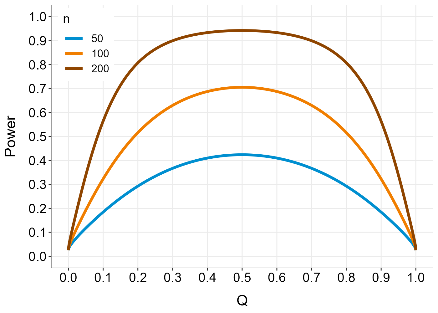
Let's compare the power curves for a comparison of two normal means with equal variances assumed to be known and significance level $\alpha = 0.05$. Assume that the absolute mean difference between the groups is $0.5$ and $\sigma = 1$. Further, let $Q = n_A/n$ so that $Q$ indicates imbalance as it goes further away from $0.5$.

PowerCurve

For large $n$, there is little loss of power for $Q$ between $0.3$ and $0.7$. The table we calculated above indicates that such a large imbalance is unlikely. However, there exist a number of restricted randomization procedures which try to protect against imbalances while also protecting against biases.

References

Rosenberger WF, Lachin JM (2016): Randomization in clinical trials: theory and practice. 2nd ed. John Wiley & Sons.

The following is adapted from section 3.2 in Rosenberger & Lachin (2016). If you have two groups and subjects are assigned to the two groups by a fair coin toss, you have complete randomization. To see why complete randomization is sometimes unattractive, let $N_A(i) = \sum_{j=1}^{i}T_j, i=1, \ldots, n$ so that $N_A(i)$ is the number of patients randomized to treatment $A$ after $i$ patients have been randomized. In the same manner, let $N_B(i) = i-N_A(i)$ be the number of patients randomized to treatment $B$. By the central limit theorem, $N_A(i)$ is asymptotically normal with mean $n/2$ and variance $n/4$. Letting $D_n=N_A(n) - N_B(n) = 2N_A(n)-n$, we see that $D_n$ is asymptotically normal with mean $0$ and variance $n$. The measure $|D_n|$ can be used to describe the degree of imbalance between the groups. For $r>0$, $$ \operatorname{Pr}(|D_n|>r)\approx 2\left\{1 - \Phi(r/\sqrt{n})\right\} $$ where $\Phi$ is the standard normal CDF.

Here is a table of the percentiles of the distribution of $|D_n|$ for complete randomization:

n <- c(50, 100, 200, 400, 800) # Vector of sample sizes
p <- c(0.33, 0.25, 0.10, 0.05, 0.025) # Vector of probabilities
# Calculate percentiles
perccr <- round(
  outer(n, p, 
      \(n, p)(qnorm(p/2, mean = 0, sd = sqrt(n), lower.tail = FALSE))
), 1)

rownames(perccr) <- n
colnames(perccr) <- p
perccr

    0.33 0.25  0.1 0.05 0.025
50   6.9  8.1 11.6 13.9  15.8
100  9.7 11.5 16.4 19.6  22.4
200 13.8 16.3 23.3 27.7  31.7
400 19.5 23.0 32.9 39.2  44.8
800 27.6 32.5 46.5 55.4  63.4

For example: When $n=200$, there is a $5\%$ probability of an imbalance of $\pm 27.7$ or worse.

The important thing to note is that imbalance does not lead to unbiased effects per se but it will decrease the precision of the estimator. Hence, imbalance will negatively affect the statistical power of the trial. But how much?

Let's compare the power curves for a comparison of two normal means with equal variances assumed to be known and significance level $\alpha = 0.05$. Assume that the absolute mean difference between the groups is $0.5$ and $\sigma = 1$. Further, let $Q = n_A/n$ so that $Q$ indicates imbalance as it goes further away from $0.5$.

PowerCurve

For large $n$, there is little loss of power for $Q$ between $0.3$ and $0.7$. The table we calculated above indicates that such a large imbalance is unlikely. However, there exist a number of restricted randomization procedures which try to protect against imbalances while also protecting against biases.

References

Rosenberger WF, Lachin JM (2016): Randomization in clinical trials: theory and practice. 2nd ed. John Wiley & Sons.

The following is adapted from section 3.2 in Rosenberger & Lachin (2016). If you have two groups and subjects are assigned to the two groups by a fair coin toss, you have complete randomization. To see why complete randomization is sometimes unattractive, let $N_A(i)$ be the number of patients randomized to treatment $A$ after $i$ patients have been randomized. In the same manner, let $N_B(i) = i-N_A(i)$ be the number of patients randomized to treatment $B$. By the central limit theorem, $N_A(i)$ is asymptotically normal with mean $n/2$ and variance $n/4$. Letting $D_n=N_A(n) - N_B(n) = 2N_A(n)-n$, we see that $D_n$ is asymptotically normal with mean $0$ and variance $n$. The measure $|D_n|$ can be used to describe the degree of imbalance between the groups. For $r>0$, $$ \operatorname{Pr}(|D_n|>r)\approx 2\left\{1 - \Phi(r/\sqrt{n})\right\} $$ where $\Phi$ is the standard normal CDF.

Here is a table of the percentiles of the distribution of $|D_n|$ for complete randomization:

n <- c(50, 100, 200, 400, 800) # Vector of sample sizes
p <- c(0.33, 0.25, 0.10, 0.05, 0.025) # Vector of probabilities
# Calculate percentiles
perccr <- round(
  outer(n, p, 
      \(n, p)(qnorm(p/2, mean = 0, sd = sqrt(n), lower.tail = FALSE))
), 1)

rownames(perccr) <- n
colnames(perccr) <- p
perccr

    0.33 0.25  0.1 0.05 0.025
50   6.9  8.1 11.6 13.9  15.8
100  9.7 11.5 16.4 19.6  22.4
200 13.8 16.3 23.3 27.7  31.7
400 19.5 23.0 32.9 39.2  44.8
800 27.6 32.5 46.5 55.4  63.4

For example: When $n=200$, there is a $5\%$ probability of an imbalance of $\pm 27.7$ or worse.

The important thing to note is that imbalance does not lead to unbiased effects per se but it will decrease the precision of the estimator. Hence, imbalance will negatively affect the statistical power of the trial. But how much?

Let's compare the power curves for a comparison of two normal means with equal variances assumed to be known and significance level $\alpha = 0.05$. Assume that the absolute mean difference between the groups is $0.5$ and $\sigma = 1$. Further, let $Q = n_A/n$ so that $Q$ indicates imbalance as it goes further away from $0.5$.

PowerCurve

For large $n$, there is little loss of power for $Q$ between $0.3$ and $0.7$. The table we calculated above indicates that such a large imbalance is unlikely. However, there exist a number of restricted randomization procedures which try to protect against imbalances while also protecting against biases.

References

Rosenberger WF, Lachin JM (2016): Randomization in clinical trials: theory and practice. 2nd ed. John Wiley & Sons.

Source Link
COOLSerdash
  • 31.2k
  • 10
  • 104
  • 157

The following is adapted from section 3.2 in Rosenberger & Lachin (2016). If you have two groups and subjects are assigned to the two groups by a fair coin toss, you have complete randomization. To see why complete randomization is sometimes unattractive, let $N_A(i) = \sum_{j=1}^{i}T_j, i=1, \ldots, n$ so that $N_A(i)$ is the number of patients randomized to treatment $A$ after $i$ patients have been randomized. In the same manner, let $N_B(i) = i-N_A(i)$ be the number of patients randomized to treatment $B$. By the central limit theorem, $N_A(i)$ is asymptotically normal with mean $n/2$ and variance $n/4$. Letting $D_n=N_A(n) - N_B(n) = 2N_A(n)-n$, we see that $D_n$ is asymptotically normal with mean $0$ and variance $n$. The measure $|D_n|$ can be used to describe the degree of imbalance between the groups. For $r>0$, $$ \operatorname{Pr}(|D_n|>r)\approx 2\left\{1 - \Phi(r/\sqrt{n})\right\} $$ where $\Phi$ is the standard normal CDF.

Here is a table of the percentiles of the distribution of $|D_n|$ for complete randomization:

n <- c(50, 100, 200, 400, 800) # Vector of sample sizes
p <- c(0.33, 0.25, 0.10, 0.05, 0.025) # Vector of probabilities
# Calculate percentiles
perccr <- round(
  outer(n, p, 
      \(n, p)(qnorm(p/2, mean = 0, sd = sqrt(n), lower.tail = FALSE))
), 1)

rownames(perccr) <- n
colnames(perccr) <- p
perccr

    0.33 0.25  0.1 0.05 0.025
50   6.9  8.1 11.6 13.9  15.8
100  9.7 11.5 16.4 19.6  22.4
200 13.8 16.3 23.3 27.7  31.7
400 19.5 23.0 32.9 39.2  44.8
800 27.6 32.5 46.5 55.4  63.4

For example: When $n=200$, there is a $5\%$ probability of an imbalance of $\pm 27.7$ or worse.

The important thing to note is that imbalance does not lead to unbiased effects per se but it will decrease the precision of the estimator. Hence, imbalance will negatively affect the statistical power of the trial. But how much?

Let's compare the power curves for a comparison of two normal means with equal variances assumed to be known and significance level $\alpha = 0.05$. Assume that the absolute mean difference between the groups is $0.5$ and $\sigma = 1$. Further, let $Q = n_A/n$ so that $Q$ indicates imbalance as it goes further away from $0.5$.

PowerCurve

For large $n$, there is little loss of power for $Q$ between $0.3$ and $0.7$. The table we calculated above indicates that such a large imbalance is unlikely. However, there exist a number of restricted randomization procedures which try to protect against imbalances while also protecting against biases.

References

Rosenberger WF, Lachin JM (2016): Randomization in clinical trials: theory and practice. 2nd ed. John Wiley & Sons.