Inspecting the coefficients of the interaction model by printing bhat2, we get these additional terms:

The only difference this time is that the last coefficient shifts the slope for the comparison group. For constructing a line for the first group, we would just get this single intercept and single slope:

Notice the first equation can be obtained simply by setting $\beta_1$ to zero, which is how we get our unconditional slope. Contrarily, inspecting the coefficients of the interaction model by printing bhat2, we get these additional terms:

The only difference this time is that the last coefficient shifts the slope for the comparison group (this is why it notes VS = 1 in the interaction term). For constructing a line for the first group, we would just get this single intercept and single slope:

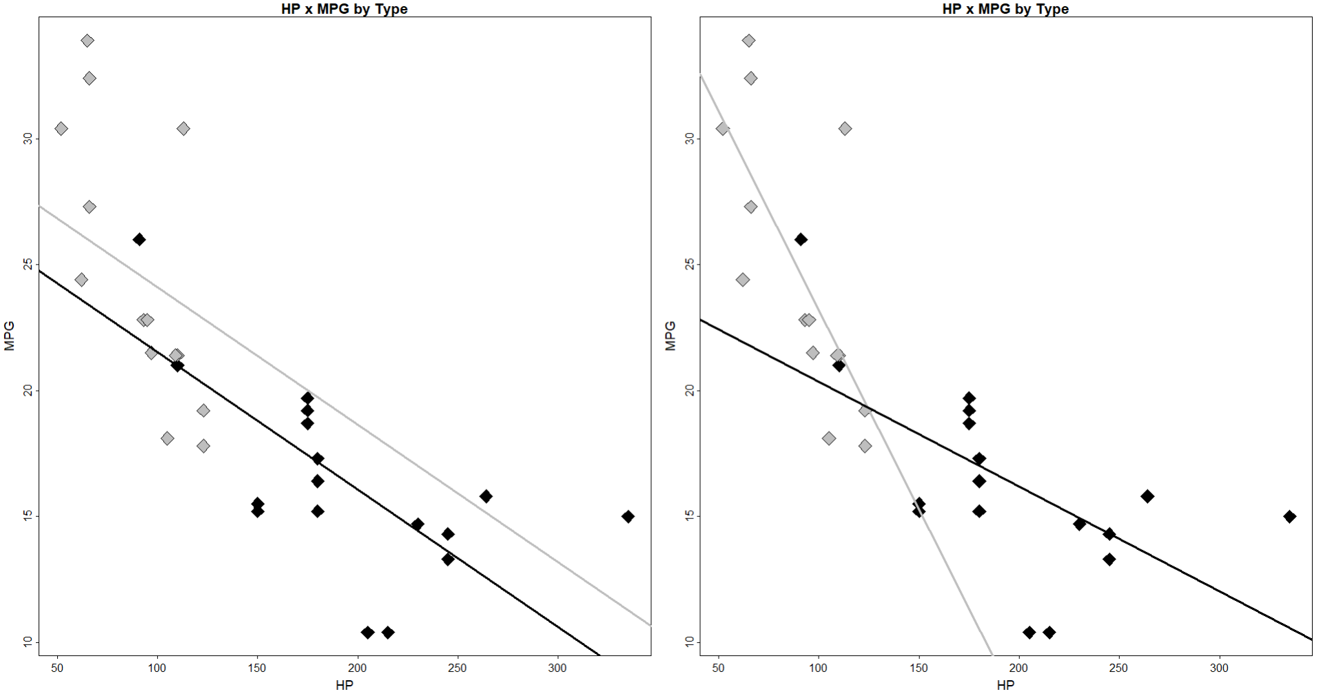
If you enter an interaction, the only difference now is that you get an adjusted slope term, which changes based on the categorical variable. One way of understanding this is comparing the plotted regression lines based on the coefficients. Below I fit a model with only main effects and another model with the interaction. Then their respective regression lines are plotted by their estimated coefficients. I use a two-level categorical variable here for simplicity by fitting the model with the mtcars data in R.

#### Main Effects Only ####
fit1 <- lm(mpg ~ factor(vs) + hp,
           mtcars)
summary(fit1)
bhat1 <- coef(fit1)
bhat1

#### Main and Interaction Effects ####
fit2 <- lm(mpg ~ factor(vs) * hp,
          mtcars)

summary(fit2)
bhat2 <- coef(fit2)
bhat2

#### Plot Main Effects Model ####
par(mfrow=c(1,2))
col <- ifelse(mtcars$vs == 0, "black","gray")

plot(mtcars$hp,
     mtcars$mpg,
     pch=23,
     bg=col,
     cex=2,
     main="HP x MPG by Type",
     xlab="HP",
     ylab="MPG")

abline(
  bhat1[1] + bhat1[2], # adjusted intercept
  bhat1[3], # unadjusted slope
  col="gray",
  lwd=3
)

abline(
  bhat1[1], # unadjusted intercept
  bhat1[3], # unadjusted slope
  col="black",
  lwd=3
)

#### Plot Interaction Model ####
plot(mtcars$hp,
     mtcars$mpg,
     pch=23,
     bg=col,
     cex=2,
     main="HP x MPG by Type",
     xlab="HP",
     ylab="MPG")

abline(
  bhat2[1] + bhat2[2], # adjusted intercept
  bhat2[3] + bhat2[4], # adjusted slope
  col="gray",
  lwd=3
)

abline(
  bhat2[1], # unadjusted intercept
  bhat2[3], # unadjusted slope
  col="black",
  lwd=3
)

Here we can see in the first model (left plot) we are simply assuming that the slope is the same between groups (hence the parallel lines), and so the only difference is the mean differences between groups (you can see the gray regression line is higher than the black one because this group has generally larger values). In the second model (right plot), we adjust each slope by group, and so the slope decreases dramatically in the black points/line.

• For the main effects-only model, the continuous predictor coefficient is the general slope, and the categorical predictor coefficient is the adjusted conditional mean (intercept).
• For the interaction model, the continuous predictor coefficient is the slope for the reference group, the categorical predictor coefficient is the adjusted conditional mean (intercept) of the comparison group, and the interaction coefficient is the adjusted value of the slope for the comparison group. So for your question:

Are the condition effects (including the intercept) interpreted as the effect when IQ=0? What is 'IQ' here?

All coefficients in the regression can be interpreted, without adjustment, as how much the outcome increases with every one unit increase in the predictor, when all other variables are set to zero. This can change if you center the variables and such. The plots should hopefully be illustrative of how this can change between main/interaction effects.

Interpreting the Coefficients

If you enter an interaction, the only difference now is that you get an adjusted slope term, which changes based on the categorical variable. Below I fit a model with only main effects and another model with the interaction. The entered variables include:

• Miles per gallon (MPG)
• Engine (VS): either v-shaped or straight
• Horsepower (HP)

I use a two-level categorical variable here for simplicity. The model is fit with the mtcars data in R. The first model is the main effects only (VS and HP) and the second model is the interaction between VS and HP.

#### Main Effects Only ####
fit1 <- lm(mpg ~ factor(vs) + hp,
           mtcars)
summary(fit1)
bhat1 <- coef(fit1)
bhat1

#### Main and Interaction Effects ####
fit2 <- lm(mpg ~ factor(vs) * hp,
          mtcars)

summary(fit2)
bhat2 <- coef(fit2)
bhat2

Inspecting the coefficients of the model with just the categorical variable and continuous variable entered as main effects only (by printing bhat1):

(Intercept) factor(vs)1          hp 
26.96300111  2.57622314 -0.05453412

The intercept (conditional mean of the reference group) is around $26.96$. The conditional mean of the comparison group (VS = 1) is higher, so its intercept is just the addition of the intercept and the factor/categorical variable's coefficient to get the adjusted intercept ($26.96 + 2.58 = 29.54$). The last coefficient is a shared slope term. When the second coefficient is set to zero, the regression line for the reference group is simply constructed as:

$$ y = (\beta_0 \times 26.96) + (\beta_2 \times -0.055) + \epsilon $$

And if we are constructing the line for the comparison group, it becomes:

$$ y = (\beta_0 \times 26.96) + (\beta_1 \times 2.58) + (\beta_2 \times -0.055) + \epsilon $$

Inspecting the coefficients of the interaction model by printing bhat2, we get these additional terms:

   (Intercept)    factor(vs)1             hp factor(vs)1:hp 
   24.49636966    14.50417652    -0.04153284    -0.11656540 

The only difference this time is that the last coefficient shifts the slope for the comparison group. For constructing a line for the first group, we would just get this single intercept and single slope:

$$ y = (\beta_0 \times 24.50) + (\beta_1 \times -0.04) + \epsilon $$

Or simply identified as:

$$ \text{intercept} = 24.50 \\ \text{slope} = -0.04 $$

For the comparison group, the regression line changes to this:

$$ y = (\beta_0 \times 24.50) + (\beta_1 \times 14.50) + (\beta_2 \times -0.04) + (\beta_3 \times -0.12) + \epsilon $$

Just like how categorical variable coefficients are simply additions to the intercept, the interaction term here is simply an addition to the slope, so it technically becomes two operations, one for the intercept and one for the slope:

$$ \text{intercept} = 24.50 + 14.50 = 39 \\ \text{slope} = -0.04 + -0.12 = -0.16 $$

Visualizing the Regression

Plots make this distinction more clear. The code for visualizing the regression in R is below:

#### Plot Main Effects Model ####
par(mfrow=c(1,2))
col <- ifelse(mtcars$vs == 0, "black","gray")

plot(mtcars$hp,
     mtcars$mpg,
     pch=23,
     bg=col,
     cex=2,
     main="HP x MPG by Type",
     xlab="HP",
     ylab="MPG")

abline(
  bhat1[1] + bhat1[2], # adjusted intercept
  bhat1[3], # unadjusted slope
  col="gray",
  lwd=3
)

abline(
  bhat1[1], # unadjusted intercept
  bhat1[3], # unadjusted slope
  col="black",
  lwd=3
)

#### Plot Interaction Model ####
plot(mtcars$hp,
     mtcars$mpg,
     pch=23,
     bg=col,
     cex=2,
     main="HP x MPG by Type",
     xlab="HP",
     ylab="MPG")

abline(
  bhat2[1] + bhat2[2], # adjusted intercept
  bhat2[3] + bhat2[4], # adjusted slope
  col="gray",
  lwd=3
)

abline(
  bhat2[1], # unadjusted intercept
  bhat2[3], # unadjusted slope
  col="black",
  lwd=3
)

Here we can see in the first model (left plot) we are simply assuming that the slope is the same between groups (hence the parallel lines), and so the only difference is the mean differences between groups (you can see the gray regression line is higher than the black one because this group has generally larger values). In the second model (right plot), we adjust each slope by group, and so the slope decreases dramatically in the gray points/line.

• For the main effects-only model, the continuous predictor coefficient is the general slope, and the categorical predictor coefficient is the adjusted conditional mean (intercept).
• For the interaction model, the continuous predictor coefficient is the slope for the reference group, the categorical predictor coefficient is the adjusted conditional mean (intercept) of the comparison group, and the interaction coefficient is the adjusted value of the slope for the comparison group.