fixed typo
Source Link

We can understand Bessel's correction geometrically by moving into $n$-dimensional space!

We will start with 3 dimensions and thethen generalize.

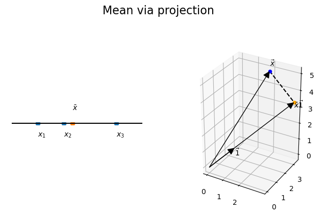
Say we have 3 observations $x_1, x_2, x_3$ of a $\mathcal{N}(\mu, \sigma^2)$ random variable. We can visualize this as $3$ points on a number line or a single vector in $\vec{x} \in \mathbb{R}^3$. A cool observation is that the mean $\bar{x}$ can be obtained geometrically by orthogonally projecting $\vec{x}$ in the direction of $\vec{1} = (1, 1,1)^\top$. In other words "The mean is the number $\bar{x}$ for which the vector $(\bar{x},\bar{x},\bar{x})^\top$ is geometrically closest to $(x_1,x_2,x_3)^\top$".

Mean via projection

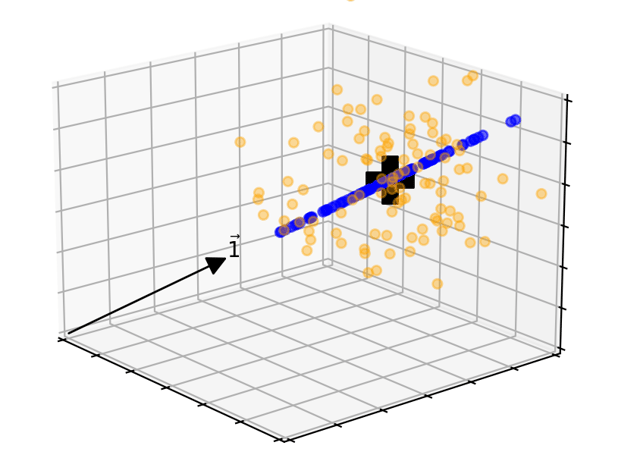
Say I generate $3$ observations $100$ times. I can visualize this as a cloud of $100$ points in $\mathbb{R}^3$. This cloud will be roughly spherical and centered at $(\mu,\mu,\mu)^\perp$. In fact, each $\vec{x}$ can be thought of as an observation from a multivariate normal $\mathcal{N}(\mu\vec{1}, \sigma^2 I_3)$.

This gives us $100$ different estimates for $\mu$. We can see this below: the $100$ yellow dots each represent a different set of $3$ observations $(x_1,x_2,x_3)$. The blue dots are their projections in the direction of $\vec{1}$ and so represent different estimates of $\mu$. The actual location of $(\mu,\mu,\mu)^\perp$ is marked with the black plus sign. It should be believable that these projections give us an unbiased estimate of $\mu$: the black plus sign should be at the center of the blue dots. So the population mean $\bar{x}$ is an unbiased estimator of the population mean $\mu$.

enter image description here

If I am only given three observations $(x_1,x_2, x_3)$ then the best I can do is estimate $\mu$ with $\bar{x}$. However I do not actually know what $\mu$ is! So I cannot use the projection of the single vector $\vec{x}$ to estimate the variance $\sigma^2$: the variance is defined as the sum of the squared deviations from $\mu$ which I do not know.

So how are we to estimate $\sigma^2$?

This is where things get tricky!

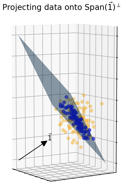
While I don't know $\mu$, I do know that $\mu\vec{1}$ and $\bar{x}\vec{1}$ are both on the same line through the origin. So if I take my orange point cloud and project it orthogonally onto $U = \textrm{span}(\vec{1})^\perp$ we know that the mean of this new blue point cloud really is $\vec{0}$! We now have a dataset with known expected value so we can actually estimate the variance!

This is a 2-dimensional collection of points drawn from a multivariate gaussian with mean $\vec{0}$ and covariance matrix $\sigma^2 I_U$.

Projection onto 1-perp

If $\vec{y} \in \mathbb{R}^k$ is an observation from $\mathcal{N}(\vec{0}, \sigma^2 I_k)$, then $\frac{1}{k} |\vec{y}|^2$ is an unbiased estimate of $\sigma^2$. This is an easy lemma:

$$ \begin{align*} \mathbb{E}\left( \frac{1}{k} |\vec{y}|^2 \right) &= \frac{1}{k} \mathbb{E} \left( \sum_1^k y_i^2\right) \\ &= \frac{1}{k} \sum_1^k \mathbb{E} \left(y_i^2\right) \\ &= \frac{1}{k} (k \sigma^2)\\ &= \sigma^2 \end{align*} $$

So, returning to our blue point cloud $\vec{x} - \bar{x}\vec{1}$ which lives on the $2$ dimensional set $U$ we get that an unbiased estimate of $\sigma^2$ would be

$$\frac{1}{2}|\vec{x} - \bar{x}\vec{1}|^2 = \frac{(x_1 - \bar{x})^2 + (x_2 - \bar{x})^2 + (x_3 - \bar{x})^2}{2}$$

We have obtained Bessel's correction!

How does this generalize to $n$ dimensions?

Exactly the same way!

Now the projection of $\vec{x} - \bar{x}\vec{1}$ lives on the $(n-1)$-dimensional subspace $\operatorname{span}(\vec{1})^\perp$. So an unbiased estimate of $\sigma^2$ is

$$ \frac{1}{n-1}|\vec{x} - \bar{x}\vec{1}|^2 = \frac{1}{n-1} \sum_1^n (x_i - \bar{x})^2 $$

This story is not exactly spelled out in the book "Statistical methods: the Geometric Approach" by David J. Saville and Graham R. Wood but it did inspire this post.

We can understand Bessel's correction geometrically by moving into $n$-dimensional space!

We will start with 3 dimensions and the generalize.

Say we have 3 observations $x_1, x_2, x_3$ of a $\mathcal{N}(\mu, \sigma^2)$ random variable. We can visualize this as $3$ points on a number line or a single vector in $\vec{x} \in \mathbb{R}^3$. A cool observation is that the mean $\bar{x}$ can be obtained geometrically by orthogonally projecting $\vec{x}$ in the direction of $\vec{1} = (1, 1,1)^\top$. In other words "The mean is the number $\bar{x}$ for which the vector $(\bar{x},\bar{x},\bar{x})^\top$ is geometrically closest to $(x_1,x_2,x_3)^\top$".

Mean via projection

Say I generate $3$ observations $100$ times. I can visualize this as a cloud of $100$ points in $\mathbb{R}^3$. This cloud will be roughly spherical and centered at $(\mu,\mu,\mu)^\perp$. In fact, each $\vec{x}$ can be thought of as an observation from a multivariate normal $\mathcal{N}(\mu\vec{1}, \sigma^2 I_3)$.

This gives us $100$ different estimates for $\mu$. We can see this below: the $100$ yellow dots each represent a different set of $3$ observations $(x_1,x_2,x_3)$. The blue dots are their projections in the direction of $\vec{1}$ and so represent different estimates of $\mu$. The actual location of $(\mu,\mu,\mu)^\perp$ is marked with the black plus sign. It should be believable that these projections give us an unbiased estimate of $\mu$: the black plus sign should be at the center of the blue dots. So the population mean $\bar{x}$ is an unbiased estimator of the population mean $\mu$.

enter image description here

If I am only given three observations $(x_1,x_2, x_3)$ then the best I can do is estimate $\mu$ with $\bar{x}$. However I do not actually know what $\mu$ is! So I cannot use the projection of the single vector $\vec{x}$ to estimate the variance $\sigma^2$: the variance is defined as the sum of the squared deviations from $\mu$ which I do not know.

So how are we to estimate $\sigma^2$?

This is where things get tricky!

While I don't know $\mu$, I do know that $\mu\vec{1}$ and $\bar{x}\vec{1}$ are both on the same line through the origin. So if I take my orange point cloud and project it orthogonally onto $U = \textrm{span}(\vec{1})^\perp$ we know that the mean of this new blue point cloud really is $\vec{0}$! We now have a dataset with known expected value so we can actually estimate the variance!

This is a 2-dimensional collection of points drawn from a multivariate gaussian with mean $\vec{0}$ and covariance matrix $\sigma^2 I_U$.

Projection onto 1-perp

If $\vec{y} \in \mathbb{R}^k$ is an observation from $\mathcal{N}(\vec{0}, \sigma^2 I_k)$, then $\frac{1}{k} |\vec{y}|^2$ is an unbiased estimate of $\sigma^2$. This is an easy lemma:

$$ \begin{align*} \mathbb{E}\left( \frac{1}{k} |\vec{y}|^2 \right) &= \frac{1}{k} \mathbb{E} \left( \sum_1^k y_i^2\right) \\ &= \frac{1}{k} \sum_1^k \mathbb{E} \left(y_i^2\right) \\ &= \frac{1}{k} (k \sigma^2)\\ &= \sigma^2 \end{align*} $$

So, returning to our blue point cloud $\vec{x} - \bar{x}\vec{1}$ which lives on the $2$ dimensional set $U$ we get that an unbiased estimate of $\sigma^2$ would be

$$\frac{1}{2}|\vec{x} - \bar{x}\vec{1}|^2 = \frac{(x_1 - \bar{x})^2 + (x_2 - \bar{x})^2 + (x_3 - \bar{x})^2}{2}$$

We have obtained Bessel's correction!

How does this generalize to $n$ dimensions?

Exactly the same way!

Now the projection of $\vec{x} - \bar{x}\vec{1}$ lives on the $(n-1)$-dimensional subspace $\operatorname{span}(\vec{1})^\perp$. So an unbiased estimate of $\sigma^2$ is

$$ \frac{1}{n-1}|\vec{x} - \bar{x}\vec{1}|^2 = \frac{1}{n-1} \sum_1^n (x_i - \bar{x})^2 $$

This story is not exactly spelled out in the book "Statistical methods: the Geometric Approach" by David J. Saville and Graham R. Wood but it did inspire this post.
We can understand Bessel's correction geometrically by moving into $n$-dimensional space!

We will start with 3 dimensions and then generalize.

Say we have 3 observations $x_1, x_2, x_3$ of a $\mathcal{N}(\mu, \sigma^2)$ random variable. We can visualize this as $3$ points on a number line or a single vector in $\vec{x} \in \mathbb{R}^3$. A cool observation is that the mean $\bar{x}$ can be obtained geometrically by orthogonally projecting $\vec{x}$ in the direction of $\vec{1} = (1, 1,1)^\top$. In other words "The mean is the number $\bar{x}$ for which the vector $(\bar{x},\bar{x},\bar{x})^\top$ is geometrically closest to $(x_1,x_2,x_3)^\top$".

Mean via projection

Say I generate $3$ observations $100$ times. I can visualize this as a cloud of $100$ points in $\mathbb{R}^3$. This cloud will be roughly spherical and centered at $(\mu,\mu,\mu)^\perp$. In fact, each $\vec{x}$ can be thought of as an observation from a multivariate normal $\mathcal{N}(\mu\vec{1}, \sigma^2 I_3)$.

This gives us $100$ different estimates for $\mu$. We can see this below: the $100$ yellow dots each represent a different set of $3$ observations $(x_1,x_2,x_3)$. The blue dots are their projections in the direction of $\vec{1}$ and so represent different estimates of $\mu$. The actual location of $(\mu,\mu,\mu)^\perp$ is marked with the black plus sign. It should be believable that these projections give us an unbiased estimate of $\mu$: the black plus sign should be at the center of the blue dots. So the population mean $\bar{x}$ is an unbiased estimator of the population mean $\mu$.

enter image description here

If I am only given three observations $(x_1,x_2, x_3)$ then the best I can do is estimate $\mu$ with $\bar{x}$. However I do not actually know what $\mu$ is! So I cannot use the projection of the single vector $\vec{x}$ to estimate the variance $\sigma^2$: the variance is defined as the sum of the squared deviations from $\mu$ which I do not know.

So how are we to estimate $\sigma^2$?

This is where things get tricky!

While I don't know $\mu$, I do know that $\mu\vec{1}$ and $\bar{x}\vec{1}$ are both on the same line through the origin. So if I take my orange point cloud and project it orthogonally onto $U = \textrm{span}(\vec{1})^\perp$ we know that the mean of this new blue point cloud really is $\vec{0}$! We now have a dataset with known expected value so we can actually estimate the variance!

This is a 2-dimensional collection of points drawn from a multivariate gaussian with mean $\vec{0}$ and covariance matrix $\sigma^2 I_U$.

Projection onto 1-perp

If $\vec{y} \in \mathbb{R}^k$ is an observation from $\mathcal{N}(\vec{0}, \sigma^2 I_k)$, then $\frac{1}{k} |\vec{y}|^2$ is an unbiased estimate of $\sigma^2$. This is an easy lemma:

$$ \begin{align*} \mathbb{E}\left( \frac{1}{k} |\vec{y}|^2 \right) &= \frac{1}{k} \mathbb{E} \left( \sum_1^k y_i^2\right) \\ &= \frac{1}{k} \sum_1^k \mathbb{E} \left(y_i^2\right) \\ &= \frac{1}{k} (k \sigma^2)\\ &= \sigma^2 \end{align*} $$

So, returning to our blue point cloud $\vec{x} - \bar{x}\vec{1}$ which lives on the $2$ dimensional set $U$ we get that an unbiased estimate of $\sigma^2$ would be

$$\frac{1}{2}|\vec{x} - \bar{x}\vec{1}|^2 = \frac{(x_1 - \bar{x})^2 + (x_2 - \bar{x})^2 + (x_3 - \bar{x})^2}{2}$$

We have obtained Bessel's correction!

How does this generalize to $n$ dimensions?

Exactly the same way!

Now the projection of $\vec{x} - \bar{x}\vec{1}$ lives on the $(n-1)$-dimensional subspace $\operatorname{span}(\vec{1})^\perp$. So an unbiased estimate of $\sigma^2$ is

$$ \frac{1}{n-1}|\vec{x} - \bar{x}\vec{1}|^2 = \frac{1}{n-1} \sum_1^n (x_i - \bar{x})^2 $$

This story is not exactly spelled out in the book "Statistical methods: the Geometric Approach" by David J. Saville and Graham R. Wood but it did inspire this post.
Source Link

We can understand Bessel's correction geometrically by moving into $n$-dimensional space!

We will start with 3 dimensions and the generalize.

Say we have 3 observations $x_1, x_2, x_3$ of a $\mathcal{N}(\mu, \sigma^2)$ random variable. We can visualize this as $3$ points on a number line or a single vector in $\vec{x} \in \mathbb{R}^3$. A cool observation is that the mean $\bar{x}$ can be obtained geometrically by orthogonally projecting $\vec{x}$ in the direction of $\vec{1} = (1, 1,1)^\top$. In other words "The mean is the number $\bar{x}$ for which the vector $(\bar{x},\bar{x},\bar{x})^\top$ is geometrically closest to $(x_1,x_2,x_3)^\top$".

Mean via projection

Say I generate $3$ observations $100$ times. I can visualize this as a cloud of $100$ points in $\mathbb{R}^3$. This cloud will be roughly spherical and centered at $(\mu,\mu,\mu)^\perp$. In fact, each $\vec{x}$ can be thought of as an observation from a multivariate normal $\mathcal{N}(\mu\vec{1}, \sigma^2 I_3)$.

This gives us $100$ different estimates for $\mu$. We can see this below: the $100$ yellow dots each represent a different set of $3$ observations $(x_1,x_2,x_3)$. The blue dots are their projections in the direction of $\vec{1}$ and so represent different estimates of $\mu$. The actual location of $(\mu,\mu,\mu)^\perp$ is marked with the black plus sign. It should be believable that these projections give us an unbiased estimate of $\mu$: the black plus sign should be at the center of the blue dots. So the population mean $\bar{x}$ is an unbiased estimator of the population mean $\mu$.

enter image description here

If I am only given three observations $(x_1,x_2, x_3)$ then the best I can do is estimate $\mu$ with $\bar{x}$. However I do not actually know what $\mu$ is! So I cannot use the projection of the single vector $\vec{x}$ to estimate the variance $\sigma^2$: the variance is defined as the sum of the squared deviations from $\mu$ which I do not know.

So how are we to estimate $\sigma^2$?

This is where things get tricky!

While I don't know $\mu$, I do know that $\mu\vec{1}$ and $\bar{x}\vec{1}$ are both on the same line through the origin. So if I take my orange point cloud and project it orthogonally onto $U = \textrm{span}(\vec{1})^\perp$ we know that the mean of this new blue point cloud really is $\vec{0}$! We now have a dataset with known expected value so we can actually estimate the variance!

This is a 2-dimensional collection of points drawn from a multivariate gaussian with mean $\vec{0}$ and covariance matrix $\sigma^2 I_U$.

Projection onto 1-perp

If $\vec{y} \in \mathbb{R}^k$ is an observation from $\mathcal{N}(\vec{0}, \sigma^2 I_k)$, then $\frac{1}{k} |\vec{y}|^2$ is an unbiased estimate of $\sigma^2$. This is an easy lemma:

$$ \begin{align*} \mathbb{E}\left( \frac{1}{k} |\vec{y}|^2 \right) &= \frac{1}{k} \mathbb{E} \left( \sum_1^k y_i^2\right) \\ &= \frac{1}{k} \sum_1^k \mathbb{E} \left(y_i^2\right) \\ &= \frac{1}{k} (k \sigma^2)\\ &= \sigma^2 \end{align*} $$

So, returning to our blue point cloud $\vec{x} - \bar{x}\vec{1}$ which lives on the $2$ dimensional set $U$ we get that an unbiased estimate of $\sigma^2$ would be

$$\frac{1}{2}|\vec{x} - \bar{x}\vec{1}|^2 = \frac{(x_1 - \bar{x})^2 + (x_2 - \bar{x})^2 + (x_3 - \bar{x})^2}{2}$$

We have obtained Bessel's correction!

How does this generalize to $n$ dimensions?

Exactly the same way!

Now the projection of $\vec{x} - \bar{x}\vec{1}$ lives on the $(n-1)$-dimensional subspace $\operatorname{span}(\vec{1})^\perp$. So an unbiased estimate of $\sigma^2$ is

$$ \frac{1}{n-1}|\vec{x} - \bar{x}\vec{1}|^2 = \frac{1}{n-1} \sum_1^n (x_i - \bar{x})^2 $$

This story is not exactly spelled out in the book "Statistical methods: the Geometric Approach" by David J. Saville and Graham R. Wood but it did inspire this post.