added 4517 characters in body
Source Link
Sextus Empiricus
  • 86.4k
  • 6
  • 115
  • 301

likelihood $\neq$ probability

The likelihood function is not the same as a probability distribution and it can be defined up to a constant.

Seperating likelihood from probability has always been tricky, already since it's introduction. In 1922 Fisher wrote in "On the Mathematical Foudations of Theoretical Statistics" about how he chose the term likelihood to make it seperate from probability

I must indeed plead guilty in my original statement of the Method of the Maximum Likelihood (9) to having based my argument upon the principle of inverse probability ; in the same paper, it is true, I emphasised the fact that such inverse probabilities were relative only. That is to say, that while we might speak of one value of as having an inverse probability three times that of another value of $p$, we might on no account introduce the differential element dp, so as to be able to say that it was three times as probable that p should lie in one rather than the other of two equal elements. Upon consideration, therefore, I perceive that the word probability is wrongly used in such a connection : probability is a ratio of frequencies, and about the frequencies of such values we can know nothing whatever. We must return to the actual fact that one value of $p$, of the frequency of which we know nothing, would yield the observed result three times as frequently as would another value of $p$. If we need a word to characterise this relative property of different values of $p$, I suggest that we may speak without confusion of the likelihood of one value of pbeing thrice the likelihood of another, bearing always in mind that likelihood is not here used loosely as a synonym of probability, but simply to express the relative frequencies with which such values of the hypothetical quantity $p$ would in fact yield the observed sample

(9) R. A. Fisher (1912). "On an Absolute Criterion for Fitting Frequency Curves,", 'Messenger of Mathematics,' xli., p. 155.

The absolute value of a likelihood is meaningless as discussed here: Is the exact value of any likelihood meaningless? An expression like "a probability of 1" has a meaning without comparing it to another probability. But an expression like "a likelihood of 1" or "a plausibility of 1", do not have the same meaning when uses without a comparison in a ratio.

TheIn the definition of likelihood function, Fisher (in On the Mathematical Foudations of Theoretical Statistics) explicitly stated that there is an arbitrary constant involved in the scale of 'likelihood'.

Likelihood — The likelihood that any parameter (or set of parameters) should have any assigned value (or set of values) is proportional to the probability that if this were so, the totality of observations should be that observed.

Distribution of likelihood

I can repeat your procedure several times and also add in the computation of the likelihood for another value of the population mean:

set.seed(123)
n = 10000
likelihood_5 = rep(NA,n)
likelihood_7 = rep(NA,n)
m_random_numbers = rep(NA,n)

for (i in 1:n) {
  random_numbers <- rnorm(50, mean = 5, sd = 5)
  m_random_numbers[i] = mean(random_numbers)
  likelihood_5[i] <- prod(dnorm(random_numbers, mean = 5, sd = 5))
  likelihood_7[i] <- prod(dnorm(random_numbers, mean = 7, sd = 5))
}

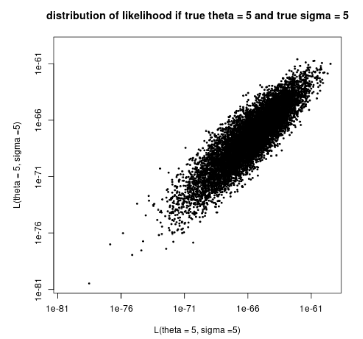
And a plot of it will look like

example of likelihood distribution

The single events that we may observe can have a very small probability. But it is not the same as a probability distributionalways a small probability. This is because the space of possible events is so large and fractionated; there are so many different events that each event has it's own small little probability.

For a likelihood it doesn't matter how probable exactly a specific event is, what matters is the distribution of likelihood and how the distribution of the likelihood for the correct model is higher than the distribution of likelihood for incorrect models.

There is an asymmetry between the probability that is used to compute a likelihood and the probability that a model has the highest likelihood. The former probabilities can be small even when the second is large.

It is not about

  • 'the probability of the event'

Instead it is but about

  • 'the probability that the likelihood of the correct model is higher'

or that

  • 'the model with the highest likelihood is with high probability close to the correct model'

Constant of proportionality

The likelihood is defined up to a constantbe proportional to the the probability of the event as function of the parameters.

This difference in a constant of proportionality is especially clear when you consider the observation of $n$ identical and independent distributed Bernoulli variables that can be either treated as a binomial distribution or a multivariate Bernoulli variable (see also In using the cbind() function in R for a logistic regression on a $2 \times 2$ table, what is the explicit functional form of the regression equation? and the same example occurs here)

An alternative view on the probability of your observation shows that the probability may actually not be as small as you think and is also diedue to additional variables that are independent from the parameter that is being investigated:

The absolute value of a likelihood is meaningless as discussed here: Is the exact value of any likelihood meaningless?

The likelihood function is also not the same as a probability distribution and it can be defined up to a constant.

This difference in a constant is especially clear when you consider the observation of $n$ identical and independent distributed Bernoulli variables that can be either treated as a binomial distribution or a multivariate Bernoulli variable (see also In using the cbind() function in R for a logistic regression on a $2 \times 2$ table, what is the explicit functional form of the regression equation?)

An alternative view on the probability of your observation shows that the probability may actually not be as small as you think and is also die to additional variables that are independent from the parameter that is being investigated:
likelihood $\neq$ probability

The likelihood function is not the same as a probability distribution and it can be defined up to a constant.

Seperating likelihood from probability has always been tricky, already since it's introduction. In 1922 Fisher wrote in "On the Mathematical Foudations of Theoretical Statistics" about how he chose the term likelihood to make it seperate from probability

I must indeed plead guilty in my original statement of the Method of the Maximum Likelihood (9) to having based my argument upon the principle of inverse probability ; in the same paper, it is true, I emphasised the fact that such inverse probabilities were relative only. That is to say, that while we might speak of one value of as having an inverse probability three times that of another value of $p$, we might on no account introduce the differential element dp, so as to be able to say that it was three times as probable that p should lie in one rather than the other of two equal elements. Upon consideration, therefore, I perceive that the word probability is wrongly used in such a connection : probability is a ratio of frequencies, and about the frequencies of such values we can know nothing whatever. We must return to the actual fact that one value of $p$, of the frequency of which we know nothing, would yield the observed result three times as frequently as would another value of $p$. If we need a word to characterise this relative property of different values of $p$, I suggest that we may speak without confusion of the likelihood of one value of pbeing thrice the likelihood of another, bearing always in mind that likelihood is not here used loosely as a synonym of probability, but simply to express the relative frequencies with which such values of the hypothetical quantity $p$ would in fact yield the observed sample

(9) R. A. Fisher (1912). "On an Absolute Criterion for Fitting Frequency Curves,", 'Messenger of Mathematics,' xli., p. 155.

The absolute value of a likelihood is meaningless as discussed here: Is the exact value of any likelihood meaningless? An expression like "a probability of 1" has a meaning without comparing it to another probability. But an expression like "a likelihood of 1" or "a plausibility of 1", do not have the same meaning when uses without a comparison in a ratio.

In the definition of likelihood, Fisher (in On the Mathematical Foudations of Theoretical Statistics) explicitly stated that there is an arbitrary constant involved in the scale of 'likelihood'.

Likelihood — The likelihood that any parameter (or set of parameters) should have any assigned value (or set of values) is proportional to the probability that if this were so, the totality of observations should be that observed.

Distribution of likelihood

I can repeat your procedure several times and also add in the computation of the likelihood for another value of the population mean:

set.seed(123)
n = 10000
likelihood_5 = rep(NA,n)
likelihood_7 = rep(NA,n)
m_random_numbers = rep(NA,n)

for (i in 1:n) {
  random_numbers <- rnorm(50, mean = 5, sd = 5)
  m_random_numbers[i] = mean(random_numbers)
  likelihood_5[i] <- prod(dnorm(random_numbers, mean = 5, sd = 5))
  likelihood_7[i] <- prod(dnorm(random_numbers, mean = 7, sd = 5))
}

And a plot of it will look like

example of likelihood distribution

The single events that we may observe can have a very small probability. But it is always a small probability. This is because the space of possible events is so large and fractionated; there are so many different events that each event has it's own small little probability.

For a likelihood it doesn't matter how probable exactly a specific event is, what matters is the distribution of likelihood and how the distribution of the likelihood for the correct model is higher than the distribution of likelihood for incorrect models.

There is an asymmetry between the probability that is used to compute a likelihood and the probability that a model has the highest likelihood. The former probabilities can be small even when the second is large.

It is not about

  • 'the probability of the event'

Instead it is but about

  • 'the probability that the likelihood of the correct model is higher'

or that

  • 'the model with the highest likelihood is with high probability close to the correct model'

Constant of proportionality

The likelihood is defined to be proportional to the the probability of the event as function of the parameters.

This difference in a constant of proportionality is especially clear when you consider the observation of $n$ identical and independent distributed Bernoulli variables that can be either treated as a binomial distribution or a multivariate Bernoulli variable (see also In using the cbind() function in R for a logistic regression on a $2 \times 2$ table, what is the explicit functional form of the regression equation? and the same example occurs here)

An alternative view on the probability of your observation shows that the probability may actually not be as small as you think and is also due to additional variables that are independent from the parameter that is being investigated:

added 6 characters in body
Source Link
Sextus Empiricus
  • 86.4k
  • 6
  • 115
  • 301

The absolute value of a likelihood is meaningless as discussed here: Is the exact value of any likelihood meaningless?

The likelihood function is also not the same as a probability distribution and it can be defined up to a constant.

This difference in a constant is especially clear when you consider the observation of $n$ identical and independent distributed Bernoulli variables that can be either treated as a binomial distribution or a multivariate Bernoulli variable (see also In using the cbind() function in R for a logistic regression on a $2 \times 2$ table, what is the explicit functional form of the regression equation?)

  • $n$ Bernoulli experiments PMF $$f(x_1,x_2,\dots,x_n) = \prod p^{x_i} (1-p)^{1-x_i} = p^{k} (1-p)^{n-k}$$
  • Binomial distribution PMF $$f(x_1,x_2,\dots,x_n) = f(k,n) = {n \choose k} p^{k} (1-p)^{n-k}$$

Here the probability for the Bernoulli experiments will be different with a factor ${n \choose k}$ from the Binomial distribution. Intuitively we can see this as the space of potential outcomes is very large (every specific order of $x_1,x_2,\dots,x_n$ is considered seperately).

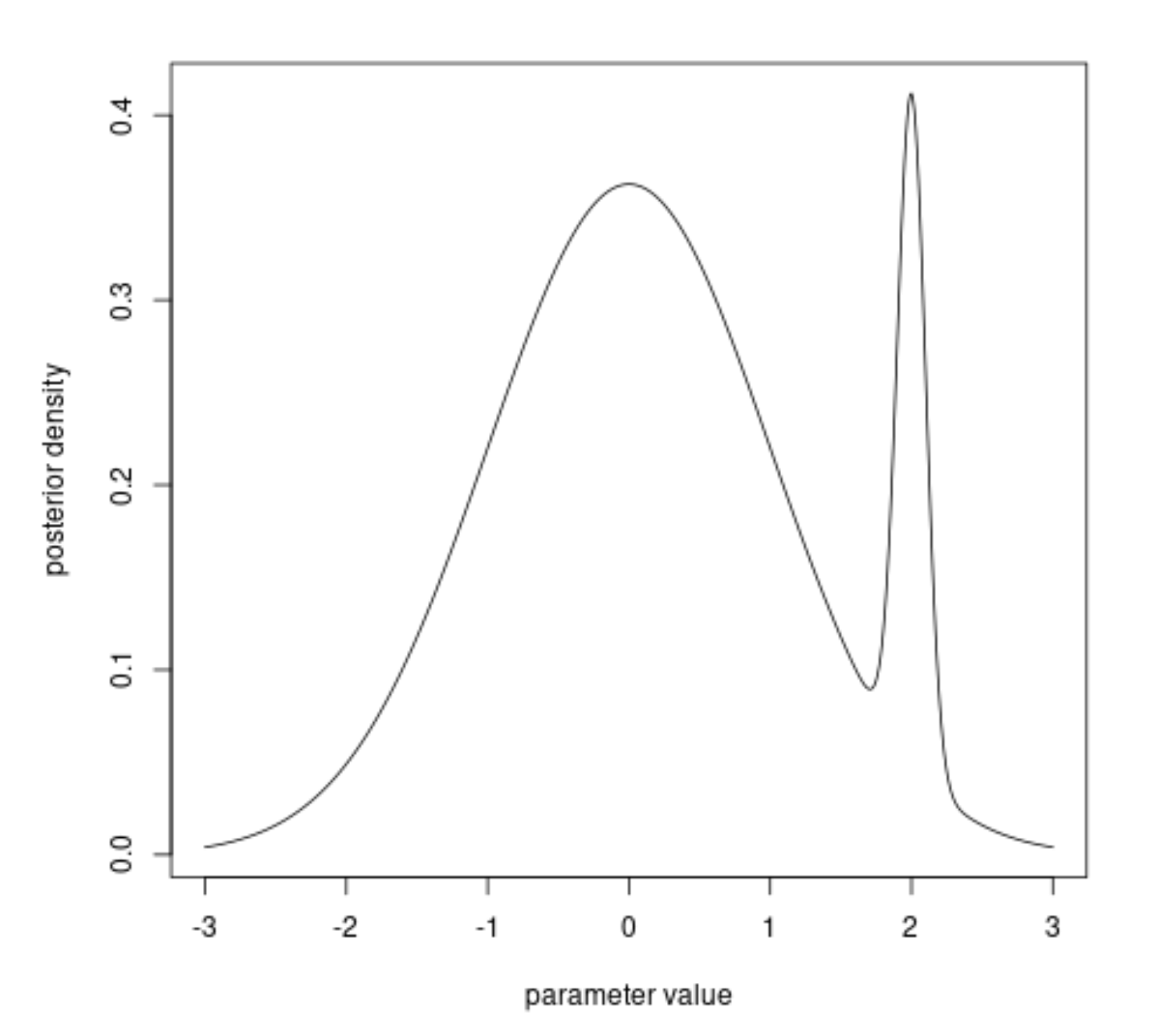
For continuous variables we even get infinitely small probabilities (see for example: Why can you not find the probability of a specific value for the normal distribution?), and you may wonder whether the absolute probability value of a single small observation is actually important. This is why often p-values are used, for a range of observations, instead of the probability of the single observed observation. An example where this can go wrong is in: Should we really search for the model for which the probability of the data is maximal? where an image like the following occurs

bi model distribution

The higher peak may not be the best estimate because the total area around it is not so large. Luckily the above is a contrived example and when we find a maximum likelihood, then this is often high for a wider entire region. Using the Fisher information (relating to the rate of change of the likelihood function) we can estimate the variance of the estimator. For likelihood functions that change slowly (are spread out a lot), we will end up with less precise estimators.


About your 10 normal distributed variables

An alternative view on the probability of your observation shows that the probability may actually not be as small as you think and is also die to additional variables that are independent from the parameter that is being investigated:

Your sample can be generated by

  • first sampling the mean in a distribution that is dependent on parameter

    $$\bar{X}|\mu \sim N\left(\mu, \frac{\sigma^2}{n}\right)$$

  • and following that sample the $X_i$ based on the value of $\bar{X}$ which follows a multivariate normal distribution that is independent from the parameter $\mu$.

    $$X_1,X_2,\dots,X_n \sim N\left(\mathbf{\bar{X}},\boldsymbol{\Sigma}\right)$$

    where $\mathbf{\bar{X}}$ is a vector with all entries equal to $\bar{X}$ and covariance matrix $\boldsymbol{\Sigma} = \sigma^2(\mathbf{I}-1/n \mathbf{J})$ (where $\mathbf{I}$ is the identitatrixidentity matrix and $\mathbf{J}$ is a matrix with all entries equal to $1$)

For the parameter $\mu$ it is only relevant what value $\bar{X}$ you observe. The exact distribution of the $X_1,X_2,\dots,X_n$ is independent from the parameter $\mu$ and irrelevant. You can add all sorts of additional variables like giving the values random colors and that would have changed the likelihood value (making it's value smaller) but it doesn't change anything about the inference of $\mu$ if these random variables have nothing to do with the value of $\mu$.

This alternative view may help to see how the actual value of the likelihood can be of less importantance, but it doesn't work in every case (e.g. when there is no sufficient statistic, like when estimating the location parameter of a Cauchy distribution)

The absolute value of a likelihood is meaningless as discussed here: Is the exact value of any likelihood meaningless?

The likelihood function is also not the same as a probability distribution and it can be defined up to a constant.

This difference in a constant is especially clear when you consider the observation of $n$ identical and independent distributed Bernoulli variables that can be either treated as a binomial distribution or a multivariate Bernoulli variable (see also In using the cbind() function in R for a logistic regression on a $2 \times 2$ table, what is the explicit functional form of the regression equation?)

  • $n$ Bernoulli experiments PMF $$f(x_1,x_2,\dots,x_n) = \prod p^{x_i} (1-p)^{1-x_i} = p^{k} (1-p)^{n-k}$$
  • Binomial distribution PMF $$f(x_1,x_2,\dots,x_n) = f(k,n) = {n \choose k} p^{k} (1-p)^{n-k}$$

Here the probability for the Bernoulli experiments will be different with a factor ${n \choose k}$ from the Binomial distribution. Intuitively we can see this as the space of potential outcomes is very large (every specific order of $x_1,x_2,\dots,x_n$ is considered seperately).

For continuous variables we even get infinitely small probabilities (see for example: Why can you not find the probability of a specific value for the normal distribution?), and you may wonder whether the absolute probability value of a single small observation is actually important. This is why often p-values are used, for a range of observations, instead of the probability of the single observed observation. An example where this can go wrong is in: Should we really search for the model for which the probability of the data is maximal? where an image like the following occurs

bi model distribution

The higher peak may not be the best estimate because the total area around it is not so large. Luckily the above is a contrived example and when we find a maximum likelihood, then this is high for a wider entire region. Using the Fisher information (relating to the rate of change of the likelihood function) we can estimate the variance of the estimator. For likelihood functions that change slowly (are spread out a lot), we will end up with less precise estimators.


About your 10 normal distributed variables

An alternative view on the probability of your observation shows that the probability may actually not be as small as you think and is also die to additional variables that are independent from the parameter that is being investigated:

Your sample can be generated by

  • first sampling the mean in a distribution that is dependent on parameter

    $$\bar{X}|\mu \sim N\left(\mu, \frac{\sigma^2}{n}\right)$$

  • and following that sample the $X_i$ based on the value of $\bar{X}$ which follows a multivariate normal distribution that is independent from the parameter $\mu$.

    $$X_1,X_2,\dots,X_n \sim N\left(\mathbf{\bar{X}},\boldsymbol{\Sigma}\right)$$

    where $\mathbf{\bar{X}}$ is a vector with all entries equal to $\bar{X}$ and covariance matrix $\boldsymbol{\Sigma} = \sigma^2(\mathbf{I}-1/n \mathbf{J})$ (where $\mathbf{I}$ is the identitatrix and $\mathbf{J}$ is a matrix with all entries equal to $1$)

For the parameter $\mu$ it is only relevant what value $\bar{X}$ you observe. The exact distribution of the $X_1,X_2,\dots,X_n$ is independent from the parameter $\mu$ and irrelevant. You can add all sorts of additional variables like giving the values random colors and that would have changed the likelihood value (making it's value smaller) but it doesn't change anything about the inference of $\mu$ if these random variables have nothing to do with the value of $\mu$.

This alternative view may help to see how the actual value of the likelihood can be of less importantance, but it doesn't work in every case (e.g. when there is no sufficient statistic, like when estimating the location parameter of a Cauchy distribution)

The absolute value of a likelihood is meaningless as discussed here: Is the exact value of any likelihood meaningless?

The likelihood function is also not the same as a probability distribution and it can be defined up to a constant.

This difference in a constant is especially clear when you consider the observation of $n$ identical and independent distributed Bernoulli variables that can be either treated as a binomial distribution or a multivariate Bernoulli variable (see also In using the cbind() function in R for a logistic regression on a $2 \times 2$ table, what is the explicit functional form of the regression equation?)

  • $n$ Bernoulli experiments PMF $$f(x_1,x_2,\dots,x_n) = \prod p^{x_i} (1-p)^{1-x_i} = p^{k} (1-p)^{n-k}$$
  • Binomial distribution PMF $$f(x_1,x_2,\dots,x_n) = f(k,n) = {n \choose k} p^{k} (1-p)^{n-k}$$

Here the probability for the Bernoulli experiments will be different with a factor ${n \choose k}$ from the Binomial distribution. Intuitively we can see this as the space of potential outcomes is very large (every specific order of $x_1,x_2,\dots,x_n$ is considered seperately).

For continuous variables we even get infinitely small probabilities (see for example: Why can you not find the probability of a specific value for the normal distribution?), and you may wonder whether the absolute probability value of a single small observation is actually important. This is why often p-values are used, for a range of observations, instead of the probability of the single observed observation. An example where this can go wrong is in: Should we really search for the model for which the probability of the data is maximal? where an image like the following occurs

bi model distribution

The higher peak may not be the best estimate because the total area around it is not so large. Luckily the above is a contrived example and when we find a maximum likelihood, then this is often high for a wider entire region. Using the Fisher information (relating to the rate of change of the likelihood function) we can estimate the variance of the estimator. For likelihood functions that change slowly (are spread out a lot), we will end up with less precise estimators.


About your 10 normal distributed variables

An alternative view on the probability of your observation shows that the probability may actually not be as small as you think and is also die to additional variables that are independent from the parameter that is being investigated:

Your sample can be generated by

  • first sampling the mean in a distribution that is dependent on parameter

    $$\bar{X}|\mu \sim N\left(\mu, \frac{\sigma^2}{n}\right)$$

  • and following that sample the $X_i$ based on the value of $\bar{X}$ which follows a multivariate normal distribution that is independent from the parameter $\mu$.

    $$X_1,X_2,\dots,X_n \sim N\left(\mathbf{\bar{X}},\boldsymbol{\Sigma}\right)$$

    where $\mathbf{\bar{X}}$ is a vector with all entries equal to $\bar{X}$ and covariance matrix $\boldsymbol{\Sigma} = \sigma^2(\mathbf{I}-1/n \mathbf{J})$ (where $\mathbf{I}$ is the identity matrix and $\mathbf{J}$ is a matrix with all entries equal to $1$)

For the parameter $\mu$ it is only relevant what value $\bar{X}$ you observe. The exact distribution of the $X_1,X_2,\dots,X_n$ is independent from the parameter $\mu$ and irrelevant. You can add all sorts of additional variables like giving the values random colors and that would have changed the likelihood value (making it's value smaller) but it doesn't change anything about the inference of $\mu$ if these random variables have nothing to do with the value of $\mu$.

This alternative view may help to see how the actual value of the likelihood can be of less importantance, but it doesn't work in every case (e.g. when there is no sufficient statistic, like when estimating the location parameter of a Cauchy distribution)

added 1240 characters in body
Source Link
Sextus Empiricus
  • 86.4k
  • 6
  • 115
  • 301

The absolute value of a likelihood is meaningless as discussed here: Is the exact value of any likelihood meaningless?

The likelihood function is also not the same as a probability distribution and it can be defined up to a constant.

This difference in a constant is especially clear when you consider the observation of $n$ identical and independent distributed Bernoulli variables that can be either treated as a binomial distribution or a multivariate Bernoulli variable (see also In using the cbind() function in R for a logistic regression on a $2 \times 2$ table, what is the explicit functional form of the regression equation?)

  • $n$ Bernoulli experiments PMF $$f(x_1,x_2,\dots,x_n) = \prod p^{x_i} (1-p)^{1-x_i} = p^{k} (1-p)^{n-k}$$
  • Binomial distribution PMF $$f(x_1,x_2,\dots,x_n) = f(k,n) = {n \choose k} p^{k} (1-p)^{n-k}$$

Here the probability for the Bernoulli experiments will be different with a factor ${n \choose k}$ from the Binomial distribution. Intuitively we can see this as the space of potential outcomes is very large (every specific order of $x_1,x_2,\dots,x_n$ is considered seperately).

For continuous variables we even get infinitely small probabilities (see for example: Why can you not find the probability of a specific value for the normal distribution?), and you may wonder whether the absolute probability value of a single small observation is actually important. This is why often p-values are used, for a range of observations, instead of the probability of the single observed observation. An example where this can go wrong is in: Should we really search for the model for which the probability of the data is maximal? where an image like the following occurs

bi model distribution

The higher peak may not be the best estimate because the total area around it is not so large. Luckily the above is a contrived example and when we find a maximum likelihood, then this is high for a wider entire region. Using the Fisher information (relating to the rate of change of the likelihood function) we can estimate the variance of the estimator. For likelihood functions that change slowly (are spread out a lot), we will end up with less precise estimators.


About your 10 normal distributed variables

An alternative view on the probability of your observation shows that the probability may actually not be as small as you think and is also die to additional variables that are independent from the parameter that is being investigated:

Your sample can be generated by

  • first sampling the mean in a distribution that is dependent on parameter

    $$\bar{X}|\mu \sim N\left(\mu, \frac{\sigma^2}{n}\right)$$

  • and following that sample the $X_i$ based on the value of $\bar{X}$ which follows a multivariate normal distribution that is independent from the parameter $\mu$.

    $$X_1,X_2,\dots,X_n \sim N\left(\mathbf{\bar{X}},\boldsymbol{\Sigma}\right)$$

    where $\mathbf{\bar{X}}$ is a vector with all entries equal to $\bar{X}$ and covariance matrix $\boldsymbol{\Sigma} = \sigma^2(\mathbf{I}-1/n \mathbf{J})$ (where $\mathbf{I}$ is the identitatrix and $\mathbf{J}$ is a matrix with all entries equal to $1$)

For the parameter $\mu$ it is only relevant what value $\bar{X}$ you observe. The exact distribution of the $X_1,X_2,\dots,X_n$ is independent from the parameter $\mu$ and irrelevant. You can add all sorts of additional variables like giving the values random colors and that would have changed the likelihood value (making it's value smaller) but it doesn't change anything about the inference of $\mu$ if these random variables have nothing to do with the value of $\mu$.

This alternative view may help to see how the actual value of the likelihood can be of less importantance, but it doesn't work in every case (e.g. when there is no sufficient statistic, like when estimating the location parameter of a Cauchy distribution)

The absolute value of a likelihood is meaningless as discussed here: Is the exact value of any likelihood meaningless?

The likelihood function is also not the same as a probability distribution and it can be defined up to a constant.

This difference in a constant is especially clear when you consider the observation of $n$ identical and independent distributed Bernoulli variables that can be either treated as a binomial distribution or a multivariate Bernoulli variable (see also In using the cbind() function in R for a logistic regression on a $2 \times 2$ table, what is the explicit functional form of the regression equation?)

  • $n$ Bernoulli experiments PMF $$f(x_1,x_2,\dots,x_n) = \prod p^{x_i} (1-p)^{1-x_i} = p^{k} (1-p)^{n-k}$$
  • Binomial distribution PMF $$f(x_1,x_2,\dots,x_n) = f(k,n) = {n \choose k} p^{k} (1-p)^{n-k}$$

Here the probability for the Bernoulli experiments will be different with a factor ${n \choose k}$ from the Binomial distribution. Intuitively we can see this as the space of potential outcomes is very large (every specific order of $x_1,x_2,\dots,x_n$ is considered seperately).

For continuous variables we even get infinitely small probabilities (see for example: Why can you not find the probability of a specific value for the normal distribution?), and you may wonder whether the absolute probability value of a single small observation is actually important. This is why often p-values are used, for a range of observations, instead of the probability of the single observed observation. An example where this can go wrong is in: Should we really search for the model for which the probability of the data is maximal? where an image like the following occurs

bi model distribution

The higher peak may not be the best estimate because the total area around it is not so large. Luckily the above is a contrived example and when we find a maximum likelihood, then this is high for a wider entire region. Using the Fisher information (relating to the rate of change of the likelihood function) we can estimate the variance of the estimator. For likelihood functions that change slowly (are spread out a lot), we will end up with less precise estimators.


About your 10 normal distributed variables

An alternative view on the probability of your observation shows that the probability may actually not be as small as you think and is also die to additional variables that are independent from the parameter that is being investigated:

Your sample can be generated by

  • first sampling the mean in a distribution that is dependent on parameter

    $$\bar{X}|\mu \sim N\left(\mu, \frac{\sigma^2}{n}\right)$$

  • and following that sample the $X_i$ based on the value of $\bar{X}$ which follows a multivariate normal distribution that is independent from the parameter $\mu$.

    $$X_1,X_2,\dots,X_n \sim N\left(\mathbf{\bar{X}},\boldsymbol{\Sigma}\right)$$

    where $\mathbf{\bar{X}}$ is a vector with all entries equal to $\bar{X}$ and covariance matrix $\boldsymbol{\Sigma} = \sigma^2(\mathbf{I}-1/n \mathbf{J})$ (where $\mathbf{I}$ is the identitatrix and $\mathbf{J}$ is a matrix with all entries equal to $1$)

For the parameter $\mu$ it is only relevant what value $\bar{X}$ you observe. The exact distribution of the $X_1,X_2,\dots,X_n$ is independent from the parameter $\mu$ and irrelevant. You can add all sorts of additional variables like giving the values random colors and that would have changed the likelihood value (making it's value smaller) but it doesn't change anything about the inference of $\mu$ if these random variables have nothing to do with the value of $\mu$.

This alternative view may help to see how the actual value of the likelihood can be of less importantance, but it doesn't work in every case (e.g. when there is no sufficient statistic, like when estimating the location parameter of a Cauchy distribution)

Source Link
Sextus Empiricus
  • 86.4k
  • 6
  • 115
  • 301
Loading