I'll start by providing the definition of comonotonicity and countermonotonicity. Then, I'll mention why this is relevant to compute the minimum and maximum possible correlation coefficient between two random variables. And finally, I'll compute these bounds for the lognormal random variables $X_1$ and $X_2$.
Comonotonicity and countermonotonicity
The random variables $X_1, \ldots, X_d$ are said to be comonotonic if their copula is the Fréchet upper bound $M(u_1, \ldots, u_d) = \min(u_1, \ldots, u_d)$, which is the strongest type of "positive" dependence.
It can be shown that $X_1, \ldots, X_d$ are comonotonic if and only if
$$
(X_1, \ldots, X_d) \stackrel{\mathrm{d}}{=} (h_1(Z), \ldots, h_d(Z)),
$$
where $Z$ is some random variable, $h_1, \ldots, h_d$ are increasing functions, and
$\stackrel{\mathrm{d}}{=}$ denotes equality in distribution.
So, comonotonic random variables are only functions of a single random variable.
The random variables $X_1, X_2$ are said to be countermonotonic if their copula is the Fréchet lower bound $W(u_1, u_2) = \max(0, u_1 + u_2 - 1)$, which is the strongest type of "negative" dependence in the bivariate case. Countermonotonocity doesn't generalize to higher dimensions.
It can be shown that $X_1, \ldots, X_d$ are countermonotonic if and only if
$$
(X_1, X_2) \stackrel{\mathrm{d}}{=} (h_1(Z), h_2(Z)),
$$
where $Z$ is some random variable, and $h_1$ and $h_2$ are respectively an increasing and a decreasing function, or vice versa.
Attaignable correlation
Let $X_1$ and $X_2$ be two random variables with strictly positive and finite variances, and let $\rho_{\rm min}$ and $\rho_{\rm max}$ denote the minimum and maximum possible correlation coefficient between $X_1$ and $X_2$.
Then, it can be shown that
- ${\rm \rho}(X_1, X_2) = \rho_{\rm min}$ if and only if $X_1$ and $X_2$ are countermonotonic;
- ${\rm \rho}(X_1, X_2) = \rho_{\rm max}$ if and only if $X_1$ and $X_2$ are comonotonic.
Attaignable correlation for lognormal random variables
To obtain $\rho_{\rm max}$ we use the fact that the maximum correlation is attained if and only if $X_1$ and $X_2$ are comonotonic. The random variables $X_1 = e^{Z}$ and $X_2 = e^{\sigma Z}$ where $Z \sim {\rm N} (0, 1)$ are comonotonic since the exponential function is a (strictly) increasing function, and thus $\rho_{\max} = {\rm corr} \left (e^Z, e^{\sigma Z} \right )$.
Using the properties of lognormal random variables, we have
${\rm E}(e^Z) = e^{1/2}$,
${\rm E}(e^{\sigma Z}) = e^{\sigma^2/2}$,
${\rm var}(e^Z) = e(e - 1)$,
${\rm var}(e^{\sigma Z}) = e^{\sigma^2}(e^{\sigma^2} - 1)$, and the covariance is
\begin{align}
{\rm cov}\left (e^Z, e^{\sigma Z}\right )
&= {\rm E}\left (e^{(\sigma + 1) Z}\right ) - {\rm E}\left (e^{\sigma Z}\right ){\rm E}\left (e^Z\right ) \\
&= e^{(\sigma + 1)^2/2} - e^{(\sigma^2 + 1)/2} \\
&= e^{(\sigma^2 + 1)/2} ( e^{\sigma} -1 ).
\end{align}
Thus,
\begin{align}
\rho_{\max}
& = \frac{ e^{(\sigma^2 + 1)/2} ( e^{\sigma} -1 ) }
{ \sqrt{ e(e - 1) e^{\sigma^2}(e^{\sigma^2} - 1) } } \\
& = \frac{ ( e^{\sigma} -1 ) }
{ \sqrt{ (e - 1) (e^{\sigma^2} - 1) } }.
\end{align}
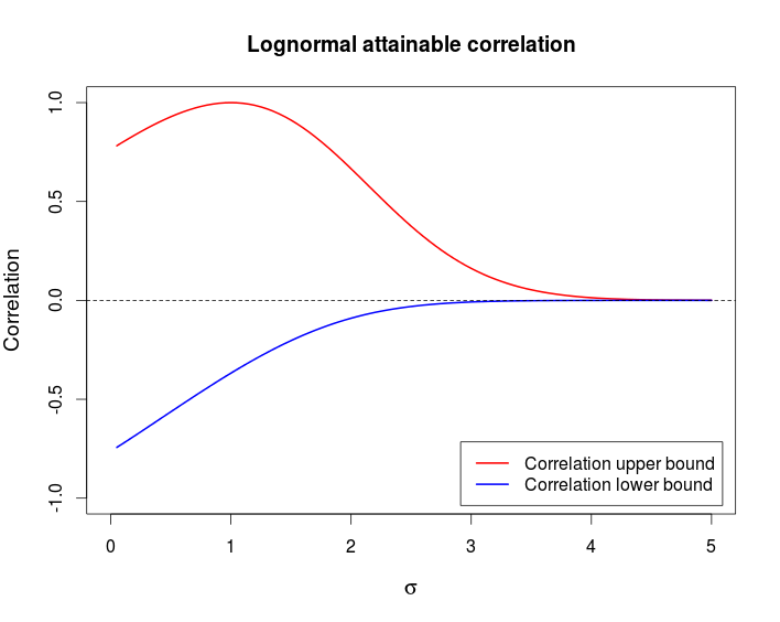
Similar computations with $X_2 = e^{-\sigma Z}$ yield
\begin{align}
\rho_{\min}
& = \frac{ ( e^{-\sigma} -1 ) }
{ \sqrt{ (e - 1) (e^{\sigma^2} - 1) } }.
\end{align}
Comment
This example shows that it is possible to have a pair of random variable that are strongly dependent - comonotonicity and countermonotonicity are the strongest kind of dependence - but that have a very low correlation.
The following chart shows these bounds as a function of $\sigma$.

This is the R code I used to produce the above chart.
curve((exp(x)-1)/sqrt((exp(1) - 1)*(exp(x^2) - 1)), from = 0, to = 5,
      ylim = c(-1, 1), col = 2, lwd = 2, main = "Lognormal attainable correlation",
      xlab = expression(sigma), ylab = "Correlation", cex.lab = 1.2)
curve((exp(-x)-1)/sqrt((exp(1) - 1)*(exp(x^2) - 1)), col = 4, lwd = 2, add = TRUE)
legend(x = "bottomright", col = c(2, 4), lwd = c(2, 2), inset = 0.02,
       legend = c("Correlation upper bound", "Correlation lower bound"))
abline(h = 0, lty = 2)

