added 920 characters in body
Source Link
whuber
  • 333.5k
  • 63
  • 792
  • 1.3k

Let $\{Y_i, i=1,2,\ldots, n\}$ be any finite collection of random variables for which

(i) $\{C\} \bigcup \{Y_i\}$ are independent and

(ii) $E[|Y_i|] \lt \infty$ for all $i.$

For $i=1, 2, \ldots,$ let $b_i:[0,1)\to \{0,1\}$ be the $i^\text{th}$ bit in the binary expansion of its argument (choosing, say, $b_i(x) = 0$ when there is more than one possible expansion, so that this is well-defined).

Define $B_i = \operatorname{sgn}(C)b_i(|C|)$$B_i = 2*b_i(|C|) - 1$ and notice that the $B_i$ are iid Rademacher variables (their values are $\pm1$ with equal probability).

The collection $X_i = B_iY_i$ does the trick:

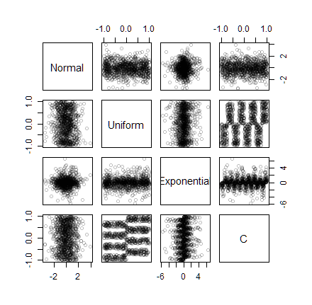
Here, to show how $C$ controls the distribution, is an illustration of a thousand realizations of $(X_1,X_2,X_3)$ using this method, starting from distributions named in the plot: enter image description here
This is the R code to produce such illustrations:

to.binary <- Vectorize(function(u, ndigits = 52) {
  bases <- 2 ^ seq_len(ndigits)
  2 * c(floor((bases * u) %% 2)) - 1 # Converts 0 and 1 to -1 and 1, resp.
}, "u")
#
# Simulate `Y` and `C` then create `X` from them.
#
n.sim <- 1e3
Y <- list(Normal = rnorm, Uniform = runif, Exponential = rexp) # The RNGs
set.seed(17)
Y.realized <- sapply(Y, \(f) f(n.sim))
C <- runif(n.sim, -1, 1)
#
# Here's the algorithm:
#
B <- t(to.binary(C, length(Y)))
X.realized <- Y.realized * B
#
# Plot the results.
#
colnames(X.realized) <- names(Y)
pairs(cbind(X.realized, C), col = "#00000040")

Let $\{Y_i, i=1,2,\ldots, n\}$ be any finite collection of random variables for which

(i) $\{C\} \bigcup \{Y_i\}$ are independent and

(ii) $E[|Y_i|] \lt \infty$ for all $i.$

For $i=1, 2, \ldots,$ let $b_i:[0,1)\to \{0,1\}$ be the $i^\text{th}$ bit in the binary expansion of its argument (choosing, say, $b_i(x) = 0$ when there is more than one possible expansion, so that this is well-defined).

Define $B_i = \operatorname{sgn}(C)b_i(|C|)$ and notice that the $B_i$ are iid Rademacher variables (their values are $\pm1$ with equal probability).

The collection $X_i = B_iY_i$ does the trick:

Let $\{Y_i, i=1,2,\ldots, n\}$ be any finite collection of random variables for which

(i) $\{C\} \bigcup \{Y_i\}$ are independent and

(ii) $E[|Y_i|] \lt \infty$ for all $i.$

For $i=1, 2, \ldots,$ let $b_i:[0,1)\to \{0,1\}$ be the $i^\text{th}$ bit in the binary expansion of its argument (choosing, say, $b_i(x) = 0$ when there is more than one possible expansion, so that this is well-defined).

Define $B_i = 2*b_i(|C|) - 1$ and notice that the $B_i$ are iid Rademacher variables (their values are $\pm1$ with equal probability).

The collection $X_i = B_iY_i$ does the trick:

Here, to show how $C$ controls the distribution, is an illustration of a thousand realizations of $(X_1,X_2,X_3)$ using this method, starting from distributions named in the plot: enter image description here

This is the R code to produce such illustrations:

to.binary <- Vectorize(function(u, ndigits = 52) {
  bases <- 2 ^ seq_len(ndigits)
  2 * c(floor((bases * u) %% 2)) - 1 # Converts 0 and 1 to -1 and 1, resp.
}, "u")
#
# Simulate `Y` and `C` then create `X` from them.
#
n.sim <- 1e3
Y <- list(Normal = rnorm, Uniform = runif, Exponential = rexp) # The RNGs
set.seed(17)
Y.realized <- sapply(Y, \(f) f(n.sim))
C <- runif(n.sim, -1, 1)
#
# Here's the algorithm:
#
B <- t(to.binary(C, length(Y)))
X.realized <- Y.realized * B
#
# Plot the results.
#
colnames(X.realized) <- names(Y)
pairs(cbind(X.realized, C), col = "#00000040")
Source Link
whuber
  • 333.5k
  • 63
  • 792
  • 1.3k

Let $\{Y_i, i=1,2,\ldots, n\}$ be any finite collection of random variables for which

(i) $\{C\} \bigcup \{Y_i\}$ are independent and

(ii) $E[|Y_i|] \lt \infty$ for all $i.$

For $i=1, 2, \ldots,$ let $b_i:[0,1)\to \{0,1\}$ be the $i^\text{th}$ bit in the binary expansion of its argument (choosing, say, $b_i(x) = 0$ when there is more than one possible expansion, so that this is well-defined).

Define $B_i = \operatorname{sgn}(C)b_i(|C|)$ and notice that the $B_i$ are iid Rademacher variables (their values are $\pm1$ with equal probability).

The collection $X_i = B_iY_i$ does the trick: