Return to Question

edited the code; starting to have doubts!

Source Link

edited Nov 24 at 7:37

library("mgcv") # mgcv_1.9-1
library("gratia") # gratia_0.9.2
## data
# some annual counts and populations (100,000s)
# the idea is to model the rate = count / 100,000 population
# n = 29 is a short time series
dat <- data.frame(time = 1996:2024,
  count = c(314, 590, 725, 953, 1218, 1688, 2227, 2751,
  3395, 4189, 4865, 5650, 5829, 6664, 7097, 8078, 8720,
  9455, 9773, 10382, 10519, 10576, 10814, 11904, 13176,
  14631, 15075, 16282, 17371),
  pop = c(23.48816, 23.81456, 24.08718, 24.39848, 24.71095,
  25.08078, 25.35108, 25.59605, 25.78745, 26.0291, 26.2812,
  26.66912, 27.13734, 27.61413, 28.0111, 28.35941, 28.73572,
  29.17764, 29.64432, 30.10587, 30.59446, 31.10672, 31.52141,
  31.9123, 32.20657, 32.11941, 32.41207, 33.22432, 34.03657))
## gam model (with negative binomial error distribution)
mod1 <- gam(count ~ offset(log(pop)) + s(time, k=14),
  data = dat, family = nb())
## simulate residuals
nn <- 29
nsims <- 2000
sims <- simulate(mod1, nsim = nsims, data = dat, unconditional=TRUE) # counts
## compute residuals and acf
# Pearson residuals are easy to compute and 
# comparable to deviance and quantile residuals for this example
lmax <- floor(10*log10(nn)) # acf() lag.max
results1 <- array(dim = c(nsims, nn)) # for residuals
results2 <- array(dim = c(nsims, lmax, 2)) # for acf
# for each simulated y
for (i in 1:nsims){
  # compute Pearson residuals = observed - simulated fit
  vars <- sims[, i] + (sims[, i]^2)/6438.266 # nb(mean, theta)
  r <- (dat$count - sims[, i]) / sqrt(vars)
  # store residual
  results1[i, ] <- r
  # compute acf and pacf
  # discard acf = 1 at lag = 0
  results2[i, , 1] <- acf(r, lag.max=lmax, plot=FALSE)$acf[2:15](lmax+1)]
  results2[i, , 2] <- pacf(r, lag.max=lmax, plot=FALSE)$acf
}
## check mean(residuals) agrees with the point estimate
rs <- matrix(nrow=nn, ncol=3)
for (i in 1:nn){
  rs[i, 1] <- mean(results1[, i])
  rs[i, 2:3] <- quantile(results1[, i], probs=c(0.025, 0.975))
}
rs <- cbind(1996:2024, rs)
rs <- as.data.frame(rs)
names(rs) <- c("time", "mean", "lower", "upper") 
r1 <- residuals(mod1, type="pearson")
# good match
plot(r1, rs$mean)
abline(0$acf
}
## check mean(residuals) agrees with the point estimate
rs <- matrix(nrow=nn, ncol=3)
for (i in 1:nn){
  rs[i, 1] <- mean(results1[, i])
  rs[i, 2:3] <- quantile(results1[, i], probs=c(0.025, 0.975))
}
rs <- cbind(dat$time, 1rs)
## summarise and plot acf
acfsrs <- matrixas.data.frame(nrow=lmax, ncol=3rs)
for names(i in 1:lmaxrs){
  acfs[i, 1] <- meanc(results2["time", i"mean", 1]"lower", "upper") 
r1 <- acfs[iresiduals(mod1, 2:3]type="pearson")
# <-good quantilematch
plot(results2[r1, irs$mean)
abline(0, 1)
## summarise and plot acf
acfs <- matrix(nrow=lmax, ncol=3)
for (i in 1:lmax){
  acfs[i, 1] <- mean(results2[, i, 1])
  acfs[i, 2:3] <- quantile(results2[, i, 1], probs=c(0.025, 0.975))
}
acfs <- cbind(dat$time, 1]acfs, probs=cacf(0.025r1, 0.975)plot=F)
}
acfs <- cbind(1:14$acf[2:(lmax+1)])
acfs <- as.data.frame(acfs)
names(acfs) <- c("lag", "mean", "lower", "upper", "acf")
plot(mean ~ lag, acfs, xlab="Lag", ylab="ACF",
    ylim=c(-0.6,0.6), lab=c(14,5,7), pch=19)
  for (i in 1:lmax){
    lines(rep(acfs[i, 1], 2), acfs[i, 3:4])
  }
  with(acfs, points(lag, acf, pch=19, col="red"))
  abline(h=0)
  abline(h=1.96/sqrt(nn), lty=2)
  abline(h=-1.96/sqrt(nn), lty=2)
  legend("topright", pch=19,
    legend=c("mean(acf p residuals)", "acf(mean(p residuals))"), col = c("black", "red"))
   ## summarise and plot pacf
pacfs <- matrix(nrow=lmax, ncol=3)
for (i in 1:lmax){
  pacfs[i, 1] <- mean(results2[, i, 2])
  pacfs[i, 2:3] <- quantile(results2[, i, 2], probs=c(0.025, 0.975))
}
pacfs <- cbind(dat$time, acfspacfs, acfpacf(r1, plot=F)$acf[2:15])
acfs <- as.data.frame(acfs)
names(acfs) <- c("lag", "mean", "lower", "upper", "acf")
plot(mean ~ lag, acfs, xlab="Lag", ylab="ACF",
    ylim=c(-0.6,0.6), lab=c(14,5,7), pch=19)
  for (i in 1:14){
    lines(rep(acfs[i, 1], 2), acfs[i, 3:4])
  }
  with(acfs, points(lag, acf, pch=19, col="red"))
  abline(h=0)
  abline(h=1.96/sqrt(29), lty=2)
  abline(h=-1.96/sqrt(29), lty=2)
  legend("topright", pch=19,
    legend=c("mean(acf p residuals)", "acf(mean(p residuals))"), col = c("black", "red"))
   ## summarise and plot pacf
pacfs <- matrix(nrow=lmax, ncol=3)
for (i in 1:lmax){
  pacfs[i, 1] <- mean(results2[, i, 2])
  pacfs[i, 2:3] <- quantile(results2[, i, 2], probs=c(0.025, 0.975))
}
pacfs <- cbind(1:14, pacfs, pacf(r1, plot=F)$acf$acf)
pacfs <- as.data.frame(pacfs)
names(pacfs) <- c("lag", "mean", "lower", "upper", "acf")
plot(mean ~ lag, pacfs, xlab="Lag", ylab="PACF",
  ylim=c(-0.6,0.6), lab=c(14,5,7), pch=19)
  for (i in 1:14lmax){
    lines(rep(pacfs[i, 1], 2), pacfs[i, 3:4])
  }
  with(pacfs, points(lag, acf, pch=19, col="red"))
  abline(h=0)
  abline(h=1.96/sqrt(29nn), lty=2)
  abline(h=-1.96/sqrt(29nn), lty=2)
  legend("topright", pch=19, legend=c("mean(pacf p residuals)", "pacf(mean(p residuals))"), col = c("black", "red"))

library("mgcv") # mgcv_1.9-1
library("gratia") # gratia_0.9.2
## data
# some annual counts and populations (100,000s)
# the idea is to model the rate = count / 100,000 population
# n = 29 is a short time series
dat <- data.frame(time = 1996:2024,
  count = c(314, 590, 725, 953, 1218, 1688, 2227, 2751,
  3395, 4189, 4865, 5650, 5829, 6664, 7097, 8078, 8720,
  9455, 9773, 10382, 10519, 10576, 10814, 11904, 13176,
  14631, 15075, 16282, 17371),
  pop = c(23.48816, 23.81456, 24.08718, 24.39848, 24.71095,
  25.08078, 25.35108, 25.59605, 25.78745, 26.0291, 26.2812,
  26.66912, 27.13734, 27.61413, 28.0111, 28.35941, 28.73572,
  29.17764, 29.64432, 30.10587, 30.59446, 31.10672, 31.52141,
  31.9123, 32.20657, 32.11941, 32.41207, 33.22432, 34.03657))
## gam model (with negative binomial error distribution)
mod1 <- gam(count ~ offset(log(pop)) + s(time, k=14),
  data = dat, family = nb())
## simulate residuals
nsims <- 2000
sims <- simulate(mod1, nsim = nsims, data = dat, unconditional=TRUE) # counts
## compute residuals and acf
# Pearson residuals are easy to compute and 
# comparable to deviance and quantile residuals for this example
lmax <- floor(10*log10(nn)) # acf() lag.max
results1 <- array(dim = c(nsims, nn)) # for residuals
results2 <- array(dim = c(nsims, lmax, 2)) # for acf
# for each simulated y
for (i in 1:nsims){
  # compute Pearson residuals = observed - simulated fit
  vars <- sims[, i] + (sims[, i]^2)/6438.266 # nb(mean, theta)
  r <- (dat$count - sims[, i]) / sqrt(vars)
  # store residual
  results1[i, ] <- r
  # compute acf and pacf
  # discard acf = 1 at lag = 0
  results2[i, , 1] <- acf(r, lag.max=lmax, plot=FALSE)$acf[2:15]
  results2[i, , 2] <- pacf(r, lag.max=lmax, plot=FALSE)$acf
}
## check mean(residuals) agrees with the point estimate
rs <- matrix(nrow=nn, ncol=3)
for (i in 1:nn){
  rs[i, 1] <- mean(results1[, i])
  rs[i, 2:3] <- quantile(results1[, i], probs=c(0.025, 0.975))
}
rs <- cbind(1996:2024, rs)
rs <- as.data.frame(rs)
names(rs) <- c("time", "mean", "lower", "upper") 
r1 <- residuals(mod1, type="pearson")
# good match
plot(r1, rs$mean)
abline(0, 1)
## summarise and plot acf
acfs <- matrix(nrow=lmax, ncol=3)
for (i in 1:lmax){
  acfs[i, 1] <- mean(results2[, i, 1])
  acfs[i, 2:3] <- quantile(results2[, i, 1], probs=c(0.025, 0.975))
}
acfs <- cbind(1:14, acfs, acf(r1, plot=F)$acf[2:15])
acfs <- as.data.frame(acfs)
names(acfs) <- c("lag", "mean", "lower", "upper", "acf")
plot(mean ~ lag, acfs, xlab="Lag", ylab="ACF",
    ylim=c(-0.6,0.6), lab=c(14,5,7), pch=19)
  for (i in 1:14){
    lines(rep(acfs[i, 1], 2), acfs[i, 3:4])
  }
  with(acfs, points(lag, acf, pch=19, col="red"))
  abline(h=0)
  abline(h=1.96/sqrt(29), lty=2)
  abline(h=-1.96/sqrt(29), lty=2)
  legend("topright", pch=19,
    legend=c("mean(acf p residuals)", "acf(mean(p residuals))"), col = c("black", "red"))
   ## summarise and plot pacf
pacfs <- matrix(nrow=lmax, ncol=3)
for (i in 1:lmax){
  pacfs[i, 1] <- mean(results2[, i, 2])
  pacfs[i, 2:3] <- quantile(results2[, i, 2], probs=c(0.025, 0.975))
}
pacfs <- cbind(1:14, pacfs, pacf(r1, plot=F)$acf)
pacfs <- as.data.frame(pacfs)
names(pacfs) <- c("lag", "mean", "lower", "upper", "acf")
plot(mean ~ lag, pacfs, xlab="Lag", ylab="PACF",
  ylim=c(-0.6,0.6), lab=c(14,5,7), pch=19)
  for (i in 1:14){
    lines(rep(pacfs[i, 1], 2), pacfs[i, 3:4])
  }
  with(pacfs, points(lag, acf, pch=19, col="red"))
  abline(h=0)
  abline(h=1.96/sqrt(29), lty=2)
  abline(h=-1.96/sqrt(29), lty=2)
  legend("topright", pch=19, legend=c("mean(pacf p residuals)", "pacf(mean(p residuals))"), col = c("black", "red"))

library("mgcv") # mgcv_1.9-1
library("gratia") # gratia_0.9.2
## data
# some annual counts and populations (100,000s)
# the idea is to model the rate = count / 100,000 population
# n = 29 is a short time series
dat <- data.frame(time = 1996:2024,
  count = c(314, 590, 725, 953, 1218, 1688, 2227, 2751,
  3395, 4189, 4865, 5650, 5829, 6664, 7097, 8078, 8720,
  9455, 9773, 10382, 10519, 10576, 10814, 11904, 13176,
  14631, 15075, 16282, 17371),
  pop = c(23.48816, 23.81456, 24.08718, 24.39848, 24.71095,
  25.08078, 25.35108, 25.59605, 25.78745, 26.0291, 26.2812,
  26.66912, 27.13734, 27.61413, 28.0111, 28.35941, 28.73572,
  29.17764, 29.64432, 30.10587, 30.59446, 31.10672, 31.52141,
  31.9123, 32.20657, 32.11941, 32.41207, 33.22432, 34.03657))
## gam model (with negative binomial error distribution)
mod1 <- gam(count ~ offset(log(pop)) + s(time, k=14),
  data = dat, family = nb())
## simulate residuals
nn <- 29
nsims <- 2000
sims <- simulate(mod1, nsim = nsims, data = dat, unconditional=TRUE) # counts
## compute residuals and acf
# Pearson residuals are easy to compute and 
# comparable to deviance and quantile residuals for this example
lmax <- floor(10*log10(nn)) # acf() lag.max
results1 <- array(dim = c(nsims, nn)) # for residuals
results2 <- array(dim = c(nsims, lmax, 2)) # for acf
# for each simulated y
for (i in 1:nsims){
  # compute Pearson residuals = observed - simulated fit
  vars <- sims[, i] + (sims[, i]^2)/6438.266 # nb(mean, theta)
  r <- (dat$count - sims[, i]) / sqrt(vars)
  # store residual
  results1[i, ] <- r
  # compute acf and pacf
  # discard acf = 1 at lag = 0
  results2[i, , 1] <- acf(r, lag.max=lmax, plot=FALSE)$acf[2:(lmax+1)]
  results2[i, , 2] <- pacf(r, lag.max=lmax, plot=FALSE)$acf
}
## check mean(residuals) agrees with the point estimate
rs <- matrix(nrow=nn, ncol=3)
for (i in 1:nn){
  rs[i, 1] <- mean(results1[, i])
  rs[i, 2:3] <- quantile(results1[, i], probs=c(0.025, 0.975))
}
rs <- cbind(dat$time, rs)
rs <- as.data.frame(rs)
names(rs) <- c("time", "mean", "lower", "upper") 
r1 <- residuals(mod1, type="pearson")
# good match
plot(r1, rs$mean)
abline(0, 1)
## summarise and plot acf
acfs <- matrix(nrow=lmax, ncol=3)
for (i in 1:lmax){
  acfs[i, 1] <- mean(results2[, i, 1])
  acfs[i, 2:3] <- quantile(results2[, i, 1], probs=c(0.025, 0.975))
}
acfs <- cbind(dat$time, acfs, acf(r1, plot=F)$acf[2:(lmax+1)])
acfs <- as.data.frame(acfs)
names(acfs) <- c("lag", "mean", "lower", "upper", "acf")
plot(mean ~ lag, acfs, xlab="Lag", ylab="ACF",
    ylim=c(-0.6,0.6), lab=c(14,5,7), pch=19)
  for (i in 1:lmax){
    lines(rep(acfs[i, 1], 2), acfs[i, 3:4])
  }
  with(acfs, points(lag, acf, pch=19, col="red"))
  abline(h=0)
  abline(h=1.96/sqrt(nn), lty=2)
  abline(h=-1.96/sqrt(nn), lty=2)
  legend("topright", pch=19,
    legend=c("mean(acf p residuals)", "acf(mean(p residuals))"), col = c("black", "red"))
   ## summarise and plot pacf
pacfs <- matrix(nrow=lmax, ncol=3)
for (i in 1:lmax){
  pacfs[i, 1] <- mean(results2[, i, 2])
  pacfs[i, 2:3] <- quantile(results2[, i, 2], probs=c(0.025, 0.975))
}
pacfs <- cbind(dat$time, pacfs, pacf(r1, plot=F)$acf)
pacfs <- as.data.frame(pacfs)
names(pacfs) <- c("lag", "mean", "lower", "upper", "acf")
plot(mean ~ lag, pacfs, xlab="Lag", ylab="PACF",
  ylim=c(-0.6,0.6), lab=c(14,5,7), pch=19)
  for (i in 1:lmax){
    lines(rep(pacfs[i, 1], 2), pacfs[i, 3:4])
  }
  with(pacfs, points(lag, acf, pch=19, col="red"))
  abline(h=0)
  abline(h=1.96/sqrt(nn), lty=2)
  abline(h=-1.96/sqrt(nn), lty=2)
  legend("topright", pch=19, legend=c("mean(pacf p residuals)", "pacf(mean(p residuals))"), col = c("black", "red"))

Source Link

asked Nov 23 at 22:56

stweb

Posterior simulation of residuals and ACF for GAMs

I am using R to smooth time series using Generalised Additive Models (GAMs).

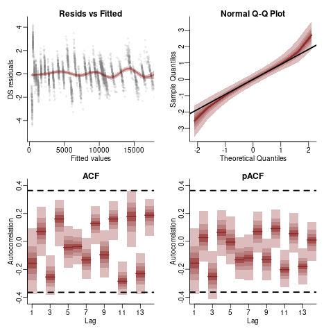
A preceding question concerned uncertain serial autocorrelation in the residuals. I was impressed by the diagnostic plots from mvgam in that:

residuals.mvgam extracts posterior draws of Dunn-Smyth (randomized quantile) residuals, and;
plot.mvgam(type="residuals") shows the variability in those draws.

The diagnostics from mgcv are more basic (and traditional) in that residuals.gam() returns point estimates.

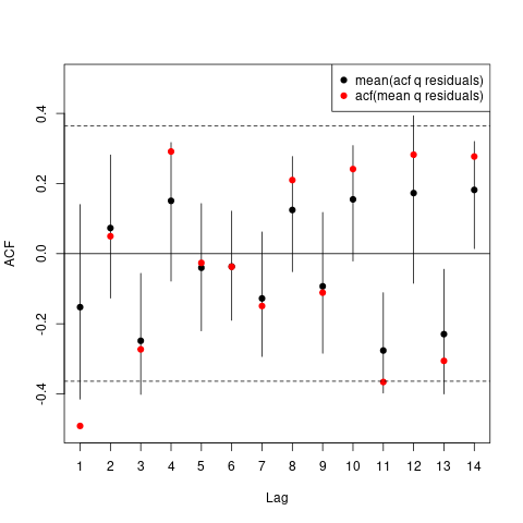
My specific concern was uncertainty about serial autocorrelation in the residuals. Examining the mvgam residuals, I found that mean(acf(residuals)) is not equal to acf(mean(residuals)), i.e. the acf() for the point estimates mean(residuals) could be insufficient for checking serial correlation. Here are two relevant plots from the previous post:

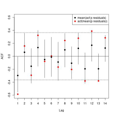
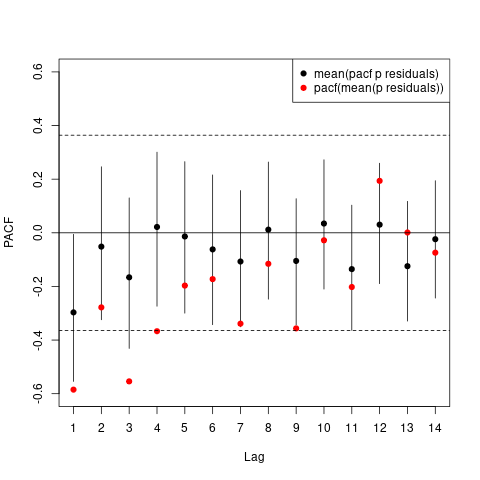
I thought to apply simulation to the mgcv::gam() model and generate serial autocorrelation diagnostics similar to those from mvgam. Below are two plots of the results and the code is below those.

The ACF plot looks similar to that for the quantile residuals above in that:

the pattern in the correlations follows that for the point estimates,
mean(acf(residuals)) is not equal to acf(mean(residuals)), and;
the 95% confidence (credibility?) intervals for the correlations are wide.

Setting aside the point estimates, the wide confidence intervals suggest that the serial autocorrelation is uncertain and largely within the tolerance interval.

Is this a reasonable (better?) method for interrogating serial autocorrelation in the residuals?

library("mgcv") # mgcv_1.9-1
library("gratia") # gratia_0.9.2
## data
# some annual counts and populations (100,000s)
# the idea is to model the rate = count / 100,000 population
# n = 29 is a short time series
dat <- data.frame(time = 1996:2024,
  count = c(314, 590, 725, 953, 1218, 1688, 2227, 2751,
  3395, 4189, 4865, 5650, 5829, 6664, 7097, 8078, 8720,
  9455, 9773, 10382, 10519, 10576, 10814, 11904, 13176,
  14631, 15075, 16282, 17371),
  pop = c(23.48816, 23.81456, 24.08718, 24.39848, 24.71095,
  25.08078, 25.35108, 25.59605, 25.78745, 26.0291, 26.2812,
  26.66912, 27.13734, 27.61413, 28.0111, 28.35941, 28.73572,
  29.17764, 29.64432, 30.10587, 30.59446, 31.10672, 31.52141,
  31.9123, 32.20657, 32.11941, 32.41207, 33.22432, 34.03657))
## gam model (with negative binomial error distribution)
mod1 <- gam(count ~ offset(log(pop)) + s(time, k=14),
  data = dat, family = nb())
## simulate residuals
nsims <- 2000
sims <- simulate(mod1, nsim = nsims, data = dat, unconditional=TRUE) # counts
## compute residuals and acf
# Pearson residuals are easy to compute and 
# comparable to deviance and quantile residuals for this example
lmax <- floor(10*log10(nn)) # acf() lag.max
results1 <- array(dim = c(nsims, nn)) # for residuals
results2 <- array(dim = c(nsims, lmax, 2)) # for acf
# for each simulated y
for (i in 1:nsims){
  # compute Pearson residuals = observed - simulated fit
  vars <- sims[, i] + (sims[, i]^2)/6438.266 # nb(mean, theta)
  r <- (dat$count - sims[, i]) / sqrt(vars)
  # store residual
  results1[i, ] <- r
  # compute acf and pacf
  # discard acf = 1 at lag = 0
  results2[i, , 1] <- acf(r, lag.max=lmax, plot=FALSE)$acf[2:15]
  results2[i, , 2] <- pacf(r, lag.max=lmax, plot=FALSE)$acf
}
## check mean(residuals) agrees with the point estimate
rs <- matrix(nrow=nn, ncol=3)
for (i in 1:nn){
  rs[i, 1] <- mean(results1[, i])
  rs[i, 2:3] <- quantile(results1[, i], probs=c(0.025, 0.975))
}
rs <- cbind(1996:2024, rs)
rs <- as.data.frame(rs)
names(rs) <- c("time", "mean", "lower", "upper") 
r1 <- residuals(mod1, type="pearson")
# good match
plot(r1, rs$mean)
abline(0, 1)
## summarise and plot acf
acfs <- matrix(nrow=lmax, ncol=3)
for (i in 1:lmax){
  acfs[i, 1] <- mean(results2[, i, 1])
  acfs[i, 2:3] <- quantile(results2[, i, 1], probs=c(0.025, 0.975))
}
acfs <- cbind(1:14, acfs, acf(r1, plot=F)$acf[2:15])
acfs <- as.data.frame(acfs)
names(acfs) <- c("lag", "mean", "lower", "upper", "acf")
plot(mean ~ lag, acfs, xlab="Lag", ylab="ACF",
    ylim=c(-0.6,0.6), lab=c(14,5,7), pch=19)
  for (i in 1:14){
    lines(rep(acfs[i, 1], 2), acfs[i, 3:4])
  }
  with(acfs, points(lag, acf, pch=19, col="red"))
  abline(h=0)
  abline(h=1.96/sqrt(29), lty=2)
  abline(h=-1.96/sqrt(29), lty=2)
  legend("topright", pch=19,
    legend=c("mean(acf p residuals)", "acf(mean(p residuals))"), col = c("black", "red"))
   ## summarise and plot pacf
pacfs <- matrix(nrow=lmax, ncol=3)
for (i in 1:lmax){
  pacfs[i, 1] <- mean(results2[, i, 2])
  pacfs[i, 2:3] <- quantile(results2[, i, 2], probs=c(0.025, 0.975))
}
pacfs <- cbind(1:14, pacfs, pacf(r1, plot=F)$acf)
pacfs <- as.data.frame(pacfs)
names(pacfs) <- c("lag", "mean", "lower", "upper", "acf")
plot(mean ~ lag, pacfs, xlab="Lag", ylab="PACF",
  ylim=c(-0.6,0.6), lab=c(14,5,7), pch=19)
  for (i in 1:14){
    lines(rep(pacfs[i, 1], 2), pacfs[i, 3:4])
  }
  with(pacfs, points(lag, acf, pch=19, col="red"))
  abline(h=0)
  abline(h=1.96/sqrt(29), lty=2)
  abline(h=-1.96/sqrt(29), lty=2)
  legend("topright", pch=19, legend=c("mean(pacf p residuals)", "pacf(mean(p residuals))"), col = c("black", "red"))