Well there are four possible approaches that come to mind (although I am sure that there are many more) but basically you could either plot the data as a perspective plot, a contour plot, a heat map or if you prefer a 3-D scatter plot (which is more or less a perspective plot when you have values of $z$ for all $(x,y)$ pairs. Here are some examples of each (from a well known 3-D data set in R):
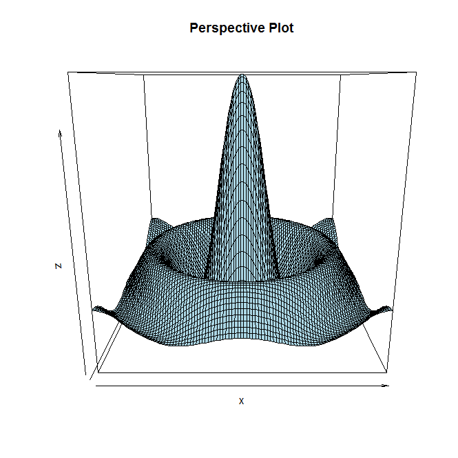
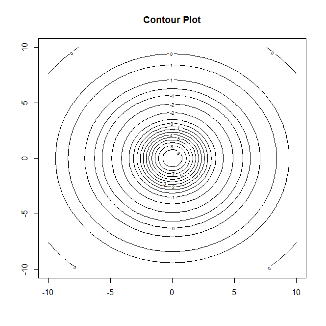
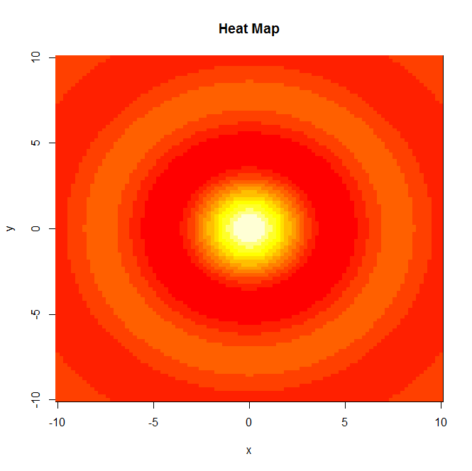
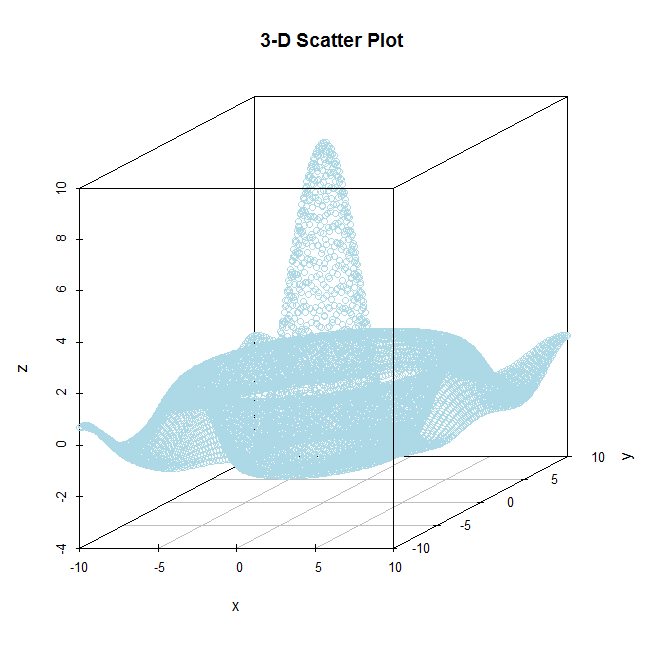
SoHere are two additional plots that have nicer plotting features than the ones given prior.
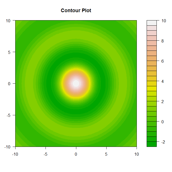
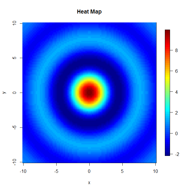 So depending on your preference will dictate which way you like to visualize 3-D data sets.
Here is the R code used to generate these four mentioned plots.
Here library(scatterplot3d)
is the `R` code
 used to generate these four mentioned plots.
library(fields)
library(scatterplot3d)

#Data for illistarition
    x = seq(-10, 10, length= 100)
    y = x
    f = function(x, y) { r = sqrt(x^2+y^2); 10 * sin(r)/r }
    z = outer(x, y, f)
    z[is.na(z)] = 1

    #Method 1
    #Perspective Plot
    persp(x,y,z,col="lightblue",main="Perspective Plot")

    #Method 2
    #Contour Plot
    contour(x,y,z,main="Contour Plot")
   filled.contour(x,y,z,color=terrain.colors,main="Contour Plot",)

#Method 3
    #Heatmap
    image(x,y,z,main="Heat Map")
   image.plot(x,y,z,main="Heat Map")

#Method 4
    #3-D Scatter Plot
    X = expand.grid(x,y)
    x = X[,1]
    y = X[,2]
    z = c(z)
    scatterplot3d(x,y,z,color="lightblue",pch=21,main="3-D Scatter Plot")
