remove 'residuals' from first sentence
Source Link
r_31415
  • 3.4k
  • 4
  • 35
  • 48

I think a good criterion is having a significant autocorrelation in the residuals in a given lag inof your data. Let me add an example taken from Cowpertwait's Introductory Time Series with R:

Suppose you have the following data and want to fit a linear model with harmonic components:

data(AirPassengers)
AP <- AirPassengers

SIN <- COS <- matrix(nr = length(AP), nc = 6)
for (i in 1:6) {
SIN[, i] <- sin(2 * pi * i * time(AP))
COS[, i] <- cos(2 * pi * i * time(AP))
}
TIME <- (time(AP) - mean(time(AP)))/sd(time(AP))
mean(time(AP))

AP.lm2 <- lm(log(AP) ~ TIME + I(TIME^2) + SIN[,1] + COS[,1] +
SIN[,2] + COS[,2] + SIN[,3] + SIN[,4] + COS[,4] + SIN[,5])

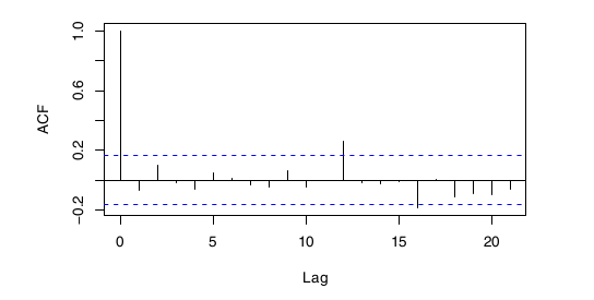
Obviously, this linear model is going to have some residuals. Calculating the autocorrelation function, you obtain the following plot (blue dotted line shows significance threshold):

AP.ar <- ar(resid(AP.lm2), order = 1, method = "mle")
enter image description here

This is telling you that there is a significant autocorrelation in lag 12 (that is, there is a correlation between each value $x_{i}$ and $x_{i+12}$ in your dataset). Therefore, you can conclude the linear model doesn't account for such seasonal variation.

In this case, the data refers to the international air passenger booking per month in an airline, so you can expected there is a seasonal variation.

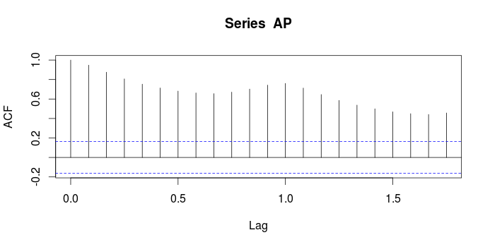
If you perform an autocorrelation on the data itself, you will see that there is a very strong autocorrelation in almost every lag (Here lag 1 means 12 months)
enter image description here

In this way, you can quantify whether or not there is a seasonal trend and how good your model is explaining such variations.

I think a good criterion is having a significant autocorrelation in the residuals in a given lag in your data. Let me add an example taken from Cowpertwait's Introductory Time Series with R:

Suppose you have the following data and want to fit a linear model with harmonic components:

data(AirPassengers)
AP <- AirPassengers

SIN <- COS <- matrix(nr = length(AP), nc = 6)
for (i in 1:6) {
SIN[, i] <- sin(2 * pi * i * time(AP))
COS[, i] <- cos(2 * pi * i * time(AP))
}
TIME <- (time(AP) - mean(time(AP)))/sd(time(AP))
mean(time(AP))

AP.lm2 <- lm(log(AP) ~ TIME + I(TIME^2) + SIN[,1] + COS[,1] +
SIN[,2] + COS[,2] + SIN[,3] + SIN[,4] + COS[,4] + SIN[,5])

Obviously, this linear model is going to have some residuals. Calculating the autocorrelation function, you obtain the following plot (blue dotted line shows significance threshold):

AP.ar <- ar(resid(AP.lm2), order = 1, method = "mle")

enter image description here

This is telling you that there is a significant autocorrelation in lag 12 (that is, there is a correlation between each value $x_{i}$ and $x_{i+12}$ in your dataset). Therefore, you can conclude the linear model doesn't account for such seasonal variation.

In this case, the data refers to the international air passenger booking per month in an airline, so you can expected there is a seasonal variation.

If you perform an autocorrelation on the data itself, you will see that there is a very strong autocorrelation in almost every lag (Here lag 1 means 12 months)

enter image description here

In this way, you can quantify whether or not there is a seasonal trend and how good your model is explaining such variations.

I think a good criterion is having a significant autocorrelation in a given lag of your data. Let me add an example taken from Cowpertwait's Introductory Time Series with R:

Suppose you have the following data and want to fit a linear model with harmonic components:

data(AirPassengers)
AP <- AirPassengers

SIN <- COS <- matrix(nr = length(AP), nc = 6)
for (i in 1:6) {
SIN[, i] <- sin(2 * pi * i * time(AP))
COS[, i] <- cos(2 * pi * i * time(AP))
}
TIME <- (time(AP) - mean(time(AP)))/sd(time(AP))
mean(time(AP))

AP.lm2 <- lm(log(AP) ~ TIME + I(TIME^2) + SIN[,1] + COS[,1] +
SIN[,2] + COS[,2] + SIN[,3] + SIN[,4] + COS[,4] + SIN[,5])

Obviously, this linear model is going to have some residuals. Calculating the autocorrelation function, you obtain the following plot (blue dotted line shows significance threshold):

AP.ar <- ar(resid(AP.lm2), order = 1, method = "mle")

enter image description here

This is telling you that there is a significant autocorrelation in lag 12 (that is, there is a correlation between each value $x_{i}$ and $x_{i+12}$ in your dataset). Therefore, you can conclude the linear model doesn't account for such seasonal variation.

In this case, the data refers to the international air passenger booking per month in an airline, so you can expected a seasonal variation.

If you perform an autocorrelation on the data itself, you will see that there is a very strong autocorrelation in almost every lag (Here lag 1 means 12 months)

enter image description here

In this way, you can quantify whether or not there is a seasonal trend and how good your model is explaining such variations.

Source Link
r_31415
  • 3.4k
  • 4
  • 35
  • 48

I think a good criterion is having a significant autocorrelation in the residuals in a given lag in your data. Let me add an example taken from Cowpertwait's Introductory Time Series with R:

Suppose you have the following data and want to fit a linear model with harmonic components:

data(AirPassengers)
AP <- AirPassengers

SIN <- COS <- matrix(nr = length(AP), nc = 6)
for (i in 1:6) {
SIN[, i] <- sin(2 * pi * i * time(AP))
COS[, i] <- cos(2 * pi * i * time(AP))
}
TIME <- (time(AP) - mean(time(AP)))/sd(time(AP))
mean(time(AP))

AP.lm2 <- lm(log(AP) ~ TIME + I(TIME^2) + SIN[,1] + COS[,1] +
SIN[,2] + COS[,2] + SIN[,3] + SIN[,4] + COS[,4] + SIN[,5])

Obviously, this linear model is going to have some residuals. Calculating the autocorrelation function, you obtain the following plot (blue dotted line shows significance threshold):

AP.ar <- ar(resid(AP.lm2), order = 1, method = "mle")

enter image description here

This is telling you that there is a significant autocorrelation in lag 12 (that is, there is a correlation between each value $x_{i}$ and $x_{i+12}$ in your dataset). Therefore, you can conclude the linear model doesn't account for such seasonal variation.

In this case, the data refers to the international air passenger booking per month in an airline, so you can expected there is a seasonal variation.

If you perform an autocorrelation on the data itself, you will see that there is a very strong autocorrelation in almost every lag (Here lag 1 means 12 months)

enter image description here

In this way, you can quantify whether or not there is a seasonal trend and how good your model is explaining such variations.